UNIVERSITÉ DE BRETAGNE OCCIDENTALE
Océanographie Physique
Pierrick Penven
Alain Colin de Verdière Directeur de thèse
Bernard Barnier Rapporteur
Geoff Brundrit Rapporteur
Xavier Carton Examinateur
Philippe Gros Examinateur
Robert Mazé Examinateur
Claude Roy Examinateur
1 décembre 2000
A numerical study of the Southern Benguela circulation
with an application to fish recruitment.
The Benguela ecosystem, along the South-west coast of Africa is, with the California
Current, the Peru-Chile and the North African upwelling systems, one of the world's 4
major ecosystems driven by an upwelling along the eastern margin of the Oceans. Their
combined total area accounts only for 0.1 % of the total surface of the world oceans,
but they provide almost 30 % of the world's total fish catch [Durand et al., 1998].
Furthermore, their yearly fluctuations explain most of the inter-annual variability of the
total marine fish catch. These fluctuations, showing years of high abundance and
dramatic collapses, result from the variability of the recruitment (which is the number
of young fish produced each year). The vulnerability of the fish larvae during the first
weeks of their lives when their displacement capabilities are limited, leaving them at
the mercy of the ocean for food accessibility or transportation, explains this large
variability in recruitment. This critical period implies that the number in a year
class is determined at a very early stage [Hjort, 1914,Hjort, 1926]. During this period, the
environment has a major impact on the survival rate of larvae. Bakun [1993] has
identified 3 classes of environmental processes that combine together to create a
favorable environment for recruitment:
- The processes of enrichment which supply the beginning of the food chain with
nutrients. They involve upwelling and vertical mixing.
- The processes of concentration, that aggregate food, eggs and larvae together.
These can occur in convergence areas such as fronts or when vertical stratification
inhibits vertical movement.
- The processes of retention that keep eggs, larvae and juveniles in a favorable
area for their survival.
In upwelling areas, the existence
of multi-variable and non-linear relationships between recruitment and
upwelling intensity is a recurrent pattern resulting from the interaction
between several environmental process [Cury and Roy, 1989,Cury et al., 1995,Durand et al., 1998].
The competition between
these different processes (enrichment, mixing, dispersion...)
leads to an "Optimal Environmental Window" that gives a
maximum for pelagic fish recruitment success in upwelling areas for a limited
averaged wind range ( 5-7 m.s
 ) [Cury and Roy, 1989].
The Benguela upwelling system is a highly dispersive environment, where a strong
equatorward wind along the coast induces an offshore displacement of the surface
waters. Although important for the enrichment of the ecosystem in nutrients, this
divergence can have a detrimental effect on the recruitment: eggs and larvae are then
carried offshore, away from their coastal habitat. In the Southern Benguela, sardines
and anchovies, the most abundant pelagic species, have adapted their reproductive
strategies to the environmental constraints. They migrate to spawn on the western
Agulhas Bank, upstream of the food sources. Eggs and larvae are advected by the currents
towards the productive areas of the West Coast of South Africa. St Helena Bay, in the
North of Cape Columbine, is recognized as the most important nursery ground of the West
Coast of South Africa [Hutchings, 1992]. This area shelters the biggest fishing industry of
the country. The loss of biological material during transport from the Agulhas Bank
to the West Coast and the retention inside the nursery ground of St Helena Bay are
supposed to be the principal factors affecting the recruitment of sardines and
anchovies [Hutchings et al., 1998].
The work presented in this manuscript is part of the VIBES (Viability of exploited
pelagic fish resources in the Benguela Ecosystems and Stocks in relation with the
environment) project. VIBES is a pluridisciplinary research project involving IRD
(Institut de Recherche pour le Développement, France), UCT (University of Cape Town,
South Africa), MCM (Marine and Coastal Management, South Africa) and LPO (Laboratoire
de Physique des Océans, France). One of the scientific goals of VIBES is to improve our
understanding of the spatial dynamics of the pelagic marine resources, the fisheries and the
environment through modeling. The present work concentrates on the modeling and the
understanding of the physical oceanic processes affecting pelagic fish recruitment in
the Southern Benguela upwelling system.
To carry out this study, we use numerical tools in order to simulate
the complex physical patterns observed in the Southern Benguela. We follow a
step by step approach. We start by setting up idealized experiments in order to
provide an understanding of the peculiarities of the circulation in St Helena Bay. At a
later stage, a 3-dimensional realistic model is implemented to reproduce the dynamics
of the ocean around the South western corner of Africa. The key processes of the
dynamics of the Southern Benguela will be identified from idealized and realistic
experiments. An analysis of these processes and a quantification of their impact on the
transport, retention and dispersion of the biological material are performed in order
to obtain the characteristic patterns affecting recruitment. The South western
corner of Africa has been much studied because of the global climate implication of the
inter-ocean exchanges that occur in this area. A high resolution model of this region
might also give new insights on the physical processes involved in the South
Atlantic-Indian Ocean exchange of properties.
The first part of the thesis concentrates on the description of the characteristic
elements of the Benguela dynamics. Numerous articles related to surveys conducted in
the Benguela upwelling system have been published during the last 30 years.
Several reviews [Nelson and Hutchings, 1983,Shannon, 1985,Shannon and Nelson, 1996,Shillington, 1998] provide a broad outline of the
observed dynamics of the Benguela. The bibliographic study conducted in this first part
of the manuscript provides a general description of the actual understanding of the
system and leads to the identification of key questions relevant to the thesis.
The second chapter presents the idealized experiments conducted to analyze the
peculiarities of the shelf circulation in St Helena Bay. The bay is situated North of
Cape Columbine, a step like variation of 100 km in the coastline. Associated with the
cape, the shelf broadens from 50 to 150 km. These topographic variations should
considerably alter the shelf dynamics. Two hypothesis are used to simplify the
problem. Firstly, the gentle slope of the shelf should allow the neglect of
processes related to stratification in the simulation of the shelf dynamics
[Clark and Brink, 1985]. Secondly, spatial and temporal wind variations are assumed to be of
secondary importance in comparison to the processes related to topography. Hence,
barotropic experiments are conducted, forced by a constant wind. These experiments are
conducted to test if a topographically induced process can balance the dispersion
caused by the wind forced coastal currents. Diagnostic tools are designed to help in the
understanding of the simulated process and a sensitivity analysis will explore the
shelf dynamics response to a range of wind forcing, bottom friction parameter and size
of the cape. An analytical solution in the form of standing shelf waves, illuminates this
important behavior of the shelf dynamics. A tracer of water age is integrated into
the model to quantify retention.
For the third chapter, a realistic regional model is implemented in order to produce a
high resolution portrayal of the ocean dynamics surrounding the
South-western corner of Africa and to explore the physical processes involved in the
different biological stages leading to recruitment, from eggs to larvae and juveniles.
A meeting organized at the beginning of the project and discussions with the different
partners of the project allowed the selection of model requirements:
- The numerical model must be able to resolve the mesoscale
features that develop over the coastal domain (like filaments, plumes, eddies, or
coastal jets...).
- The model domain must include the main pelagic fish spawning and nursery
grounds.
- It must be large enough to allow the relevant physical processes to fully
develop, but small enough to obtain sufficient fine spatial resolution at a
reasonable computational cost.
The Benguela upwelling system is unique in a way that the
African continent ends at around 34 S. This induces the highly energetic poleward
termination of the western boundary current of the Indian Ocean, the Agulhas Current,
to flow along the Agulhas Bank and somehow to interact with the Benguela upwelling
system. It retroflects South of the Agulhas Bank to flow back into the Indian Ocean. One
should note that the anticyclonic eddies shed at the retroflection area, the Agulhas
rings, are the biggest coherent structures observed in the Ocean. The handling of these
highly energetic structures and currents by a regional oceanic model of finite dimension
is a challenge that require specific treatments. Recently, long term simulations (of more
than 10 years) have been conducted using a regional oceanic model for the California
Current System [Marchesiello et al., 2000]. The model employed is ROMS, the Regional Ocean Modeling
System. It uses a generalized nonlinear terrain-following coordinate, high order schemes
and new parameterizations that have been especially implemented to resolve with a high
level of accuracy the primitive equation of momentum along the shelf and the slope on a
regional scale. Though there is no equivalent of the Agulhas Current along the West
Coast of the United States, we expect to obtain long-term meaningful results using the
same tool for the Benguela upwelling system. The validation of the model results will be
done through comparison with data. The study of the variability of the system and of
typical mesoscale processes will give insights for the understanding of the Benguela
dynamics. Special attention is given to the model solution on the shelves along the
South and West coasts, and comparison is also made with the results of the idealized
experiments. If the realistic model solution is satisfactory, it will be possible to use
the model to explore transport mechanisms from the Agulhas Bank to West Coast and
retention processes in the coastal domain. This is done by introducing a passive
tracer that simulates eggs and larvae transport behavior.
S. This induces the highly energetic poleward
termination of the western boundary current of the Indian Ocean, the Agulhas Current,
to flow along the Agulhas Bank and somehow to interact with the Benguela upwelling
system. It retroflects South of the Agulhas Bank to flow back into the Indian Ocean. One
should note that the anticyclonic eddies shed at the retroflection area, the Agulhas
rings, are the biggest coherent structures observed in the Ocean. The handling of these
highly energetic structures and currents by a regional oceanic model of finite dimension
is a challenge that require specific treatments. Recently, long term simulations (of more
than 10 years) have been conducted using a regional oceanic model for the California
Current System [Marchesiello et al., 2000]. The model employed is ROMS, the Regional Ocean Modeling
System. It uses a generalized nonlinear terrain-following coordinate, high order schemes
and new parameterizations that have been especially implemented to resolve with a high
level of accuracy the primitive equation of momentum along the shelf and the slope on a
regional scale. Though there is no equivalent of the Agulhas Current along the West
Coast of the United States, we expect to obtain long-term meaningful results using the
same tool for the Benguela upwelling system. The validation of the model results will be
done through comparison with data. The study of the variability of the system and of
typical mesoscale processes will give insights for the understanding of the Benguela
dynamics. Special attention is given to the model solution on the shelves along the
South and West coasts, and comparison is also made with the results of the idealized
experiments. If the realistic model solution is satisfactory, it will be possible to use
the model to explore transport mechanisms from the Agulhas Bank to West Coast and
retention processes in the coastal domain. This is done by introducing a passive
tracer that simulates eggs and larvae transport behavior.
Following this approach, we expect to provide a better understanding of the dynamics of
the Southern Benguela as well as necessary tools for the ongoing study of the dynamics
of the recruitment.
1 The Benguela
The fisheries of the South African West Coast being of large
economical importance, an important effort has been directed by South
African marine research institutes to analyze the ecosystem. Thus, numerous
studies have been undertaken in the last 30 years, involving for the physical
part: hydrological samplings, current meters deployments, aerial atmospheric
and sea surface temperature measurements, ADCP current measurements, drifters
deployments, satellite data analysis and theoretical studies. As a result, a
thorough description of the system is available and the understanding of many
important processes has significantly progressed. These results have been
summarized in several reviews [Nelson and Hutchings, 1983,Shannon, 1985,Shannon and Nelson, 1996,Shillington, 1998].
The aim of this chapter is to produce a general description of the Benguela
system and its peculiarities. A more specific goal is to identify the
characteristic patterns of the Benguela dynamics and to extract the key
processes that affect the recruitment of sardines and anchovies along the
South African West Coast. This analysis leads to the identification of a
few key questions relevant for this study.
Les pêcheries le long de la Côte Ouest de l'Afrique du Sud étant d'une
importance économique majeure, un effort considérable a été
réalisé par
les instituts de recherches marines Sud-africains pour analyser
l'écosystême du Benguela.
Ainsi, de nombreuses études ont été conduites durant les 30 dernières
années, comprenant pour la partie physique: des échantillonages
hydrologiques, le déploiement de mouillages courantométriques,
des mesures aériennes des composantes atmosphériques et de la température
de surface de l'eau, des mesures courantométriques par ADCP, le larguage de
flotteurs dérivants, l'analyse d'images satellitales, et des études
théoriques.
Il en découle une descrition détaillée du système; et des
progrès significatifs ont été obtenus dans la compréhension des
principaux processus. Ces résultats ont été résumés dans
différentes revues d'articles [Nelson and Hutchings, 1983,Shannon, 1985,Shannon and Nelson, 1996,Shillington, 1998].
L'objectif de ce chapitre est de produire une descripton générale du
système du Benguela et de ses particularités. Un but plus précis est
l'identification des motifs caractéristiques de la dynamique du Benguela
et d'extraire les processus clefs pouvant affecter le recrutement des
sardines et des anchois le long de la Côte Ouest de l'Afrique du Sud.
Cette analyse conduit à la formulation de quelques questions clefs,
pertinantes pour cette étude.
1 Geographical settings
Figure 1.1:
Surface currents of the South Atlantic Ocean. Abbreviations are used
for the Angola-Benguela Front (ABF), Brazil Current Front (BCF), Sub-tropical
Front (STF), Sub-antarctic Front (SAF), Polar Front (PF) and Continental Water
Boundary / Wedell Gyre Boundary (CWB/WGB). Adapted from Tomczak and
Godfrey [1994].
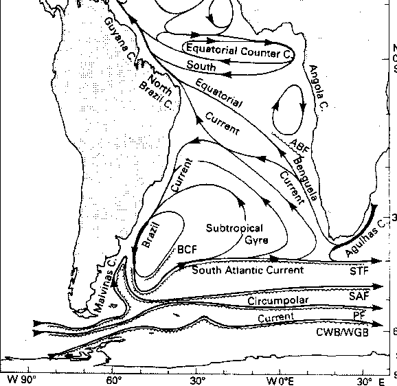 |
The Benguela Current is the eastern boundary current of the South Atlantic
sub-tropical gyre
[Peterson and Stramma, 1987] (figure 1.1). It can be
described as a broad northward flow that follows the west coast of southern
Africa from the southern tip of Africa (i.e. the Cape Agulhas at 35 S) to
Cape Frio ( S) near the border between Angola and Namibia [Garzoli and Gordon, 1996].
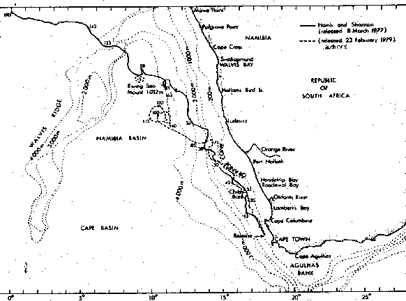
The similar paths of 2 drifters released near Cape Peninsula with an interval of
two years exhibit the coherent equatorward surface movement of the current
(figure 1.2) [Nelson and Hutchings, 1983].
S) near the border between Angola and Namibia [Garzoli and Gordon, 1996].
The similar paths of 2 drifters released near Cape Peninsula with an interval of
two years exhibit the coherent equatorward surface movement of the current
(figure 1.2) [Nelson and Hutchings, 1983].
Figure 1.2:
Paths of two satellite-tracked drogues released west of Cape Town in
March 1977 and in February 1979. Adapted from Nelson and Hutchings [1983].
 |
The Benguela system is bounded in the North at about  S by the
warm Angolan current, which flows poleward. It is bounded in the South by the warm
Agulhas Current, the western boundary current of the Indian Ocean
that follows the South Coast of South Africa [Shillington, 1998]. The terminology
"Benguela Current" describes as well the coastal upwelling system and the large
scale eastern limb of the sub-tropical gyre [Peterson and Stramma, 1987], thus no precise
offshore boundary of the system is defined. For Garzoli and Gordon [1996], at
S by the
warm Angolan current, which flows poleward. It is bounded in the South by the warm
Agulhas Current, the western boundary current of the Indian Ocean
that follows the South Coast of South Africa [Shillington, 1998]. The terminology
"Benguela Current" describes as well the coastal upwelling system and the large
scale eastern limb of the sub-tropical gyre [Peterson and Stramma, 1987], thus no precise
offshore boundary of the system is defined. For Garzoli and Gordon [1996], at
 S, the entire Benguela Current is confined between the South African
West Coast and the Walvis ridge (
S, the entire Benguela Current is confined between the South African
West Coast and the Walvis ridge ( km from the coast). In this
manuscript, we will limit our definition of the Benguela Current to the part of
the current that flows over the shelf and the continental slope.
km from the coast). In this
manuscript, we will limit our definition of the Benguela Current to the part of
the current that flows over the shelf and the continental slope.
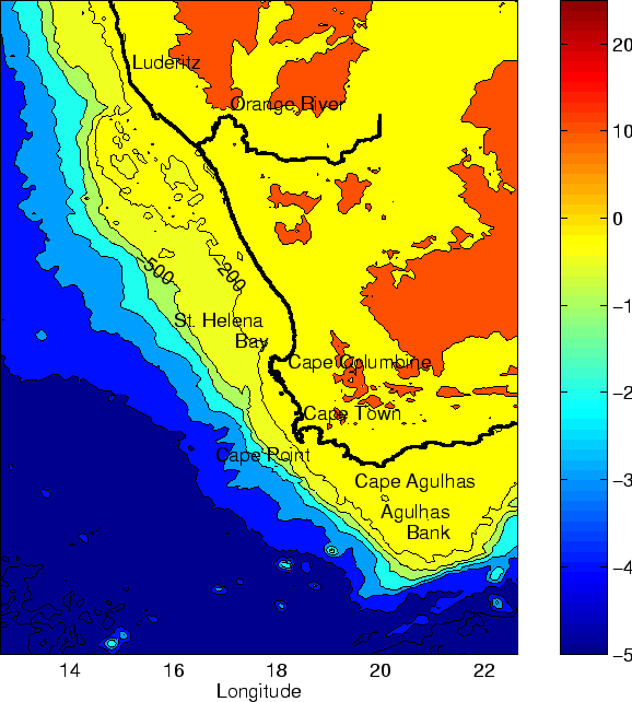
Figure 1.3:
Bathymetry of the South-east Atlantic Ocean derived from the ETOPO2
dataset.
 |
The West Coast of Southern Africa is a narrow coastal plain which rises to the
main continental escarpment situated between 50 and 200 km inland.
North of  S (Cape Columbine), the coastline is regular and runs in a
north-westward direction. South of S the coastline is
irregular, with several capes (Cape Columbine S, Cape Peninsula
S (Cape Columbine), the coastline is regular and runs in a
north-westward direction. South of S the coastline is
irregular, with several capes (Cape Columbine S, Cape Peninsula  S,
Cape Agulhas
S,
Cape Agulhas  S) and bays (St Helena bay, Saldanha Bay, Table Bay, False
Bay). One thousand meters-high mountains ranging along the Cape Peninsula can play an
important role in perturbing the local wind field [Shannon, 1985].
Most of the coastal region is arid with the Namib Desert that extends between
S) and bays (St Helena bay, Saldanha Bay, Table Bay, False
Bay). One thousand meters-high mountains ranging along the Cape Peninsula can play an
important role in perturbing the local wind field [Shannon, 1985].
Most of the coastal region is arid with the Namib Desert that extends between
 S and
S and  S. The southern region has a cooler Mediterranean type
climate.
The continental shelf is highly variable in width (figure 1.3).
It can be narrow with minimums located South of Lüderitz (75 km) and in front
of Cape Peninsula (40 km), and it can be relatively wide with maximums located
off the Orange river (180 km) and on the Agulhas Bank (230 km). The shelf break
is deep (200 m) and quasi-rectilinear, running North westward roughly parallel
to the coast. It is cut in a north-south direction at 60 km offshore of Cape Columbine by
the Cape Canyon. The Agulhas Bank is a wide and shallow feature that forms the
southernmost margin of the African continent [Shannon and Nelson, 1996].
S. The southern region has a cooler Mediterranean type
climate.
The continental shelf is highly variable in width (figure 1.3).
It can be narrow with minimums located South of Lüderitz (75 km) and in front
of Cape Peninsula (40 km), and it can be relatively wide with maximums located
off the Orange river (180 km) and on the Agulhas Bank (230 km). The shelf break
is deep (200 m) and quasi-rectilinear, running North westward roughly parallel
to the coast. It is cut in a north-south direction at 60 km offshore of Cape Columbine by
the Cape Canyon. The Agulhas Bank is a wide and shallow feature that forms the
southernmost margin of the African continent [Shannon and Nelson, 1996].
2 Large scale
The Benguela current flows northward from the Cape of Good Hope. It bends
towards the northwest to separate from the coast at around S while
widening rapidly [Peterson and Stramma, 1987].
Three currents are feeding the Benguela Current: the South Atlantic Current,
which is the southern part of the sub-tropical gyre, the Agulhas current and the
Antarctic Circumpolar Current. The composition of the Benguela Current water
is as follows: 50  of Atlantic water, 25 of water from the Indian
Ocean and 25 of a blend of Agulhas and tropical Atlantic water
[Garzoli and Gordon, 1996].
of Atlantic water, 25 of water from the Indian
Ocean and 25 of a blend of Agulhas and tropical Atlantic water
[Garzoli and Gordon, 1996].
Figure 1.4:
The principal water masses and potential temperature - salinity
characteristics of the South-east Atlantic and Benguela system. Adapted from Shannon
and Nelson [1996].
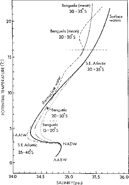 |
A T-S diagram exposes the hydrological characteristics of the principal water
masses in the Benguela system (figure 1.4). The surface waters are
composed of tropical surface water and subtropic surface water. Three kinds of
thermocline waters are present: the South Atlantic Central Water (SACW), the
South Indian Central Water (SICW) and the Tropical Atlantic Central Water
(TACW). Under these, the fresh Antarctic Intermediate Water (AAIW),
characteristic of the South-East Atlantic Ocean by its core of minimum of
salinity around 700-800 m, flows toward the equator [Shannon and Nelson, 1996]. 4-5 Sv of
AAIW is carried this way northward in the Benguela. Underneath, the relatively
warm and saline North Atlantic Deep Water (NADW) spreads southward from the
North Atlantic between 1000 m and 3500 m. It generates a poleward current along
the African continental margin. The Antarctic Bottom Water (AABW) lies below
the NADW under 3800 m. Blocked in the North by the Walvis ridge (figure
1.3) , the circulation of the AABW in the Cape Basin is
cyclonic. Thus the AABW produces as well a poleward current along the African
continental margin with typical speeds of 5 to 10 cm.s [Nelson, 1989].
Figure 1.5:
Schematic flow field of surface and thermocline waters. Current
speeds refer to surface values. Transports (circled) refers to total
transport above 1500 db (i.e. includes AAIW). Adapted from Shannon and Nelson
[1996].
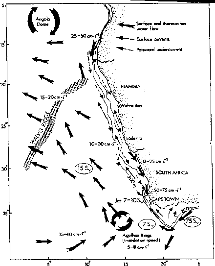 |
Equatorward flow occurs in the surface to depth of several hundred of meters.
In the surface friction layer, the Ekman drift is typically 20 to 35
cm.s [Nelson, 1989]. Recent measurements showed that in the upper 1000 m,
the Benguela current carries 13 Sv towards the equator across S
[Garzoli and Gordon, 1996]. The upper layers averaged circulation and transport is summarized
in figure 1.5.
One can note in figure (1.5) the large transport (75 Sv) carried by to
the Agulhas Current, the western boundary current of the Indian Ocean
subtropical gyre, just South-East of the Benguela system. As it flows along the
South and East coasts of South Africa, the Agulhas Current reaches an intensity
unmatched by any other western boundary currents [Beal and Bryden, 1997] at up to 6 knots
(300 cm.s) [Boyd and Oberholster, 1994]. Its follows the shelf break along the eastern
margin of the Agulhas Bank, developing meanders, reverse plumes and counter
current on the shelf [Lutjeharms et al., 1989]. It generally leaves the coast just East of
the tip of the Agulhas Bank before turning back on itself and flowing eastward
into the South Indian Ocean. In this retroflection area, the largest eddies
found in the oceans (with diameters up to 300 km), the Agulhas rings, detach
from the current and transport warm and salty waters into the South Atlantic.
They account for a time-averaged transfer of 10-15 Sv in the upper 1000 m and
thus play an important part in the global thermohaline circulation
[Peterson and Stramma, 1987]. Regularly, warm filaments detach from the southern tip of the
Agulhas Bank and develop into the Benguela system [Lutjeharms and Cooper, 1996]. Along the East
coast of South Africa ( S) the presence of a persistent Agulhas
undercurrent with velocities as large as 30 cm.s and a core at depth
around 1200 m has been recently measured [Beal and Bryden, 1997].
3 Atmospheric forcing
Figure 1.6:
Mean atmospheric sea level pressure (hpa) for (a) January, and (b)
July. Adapted from Peterson and Stramma [1987].
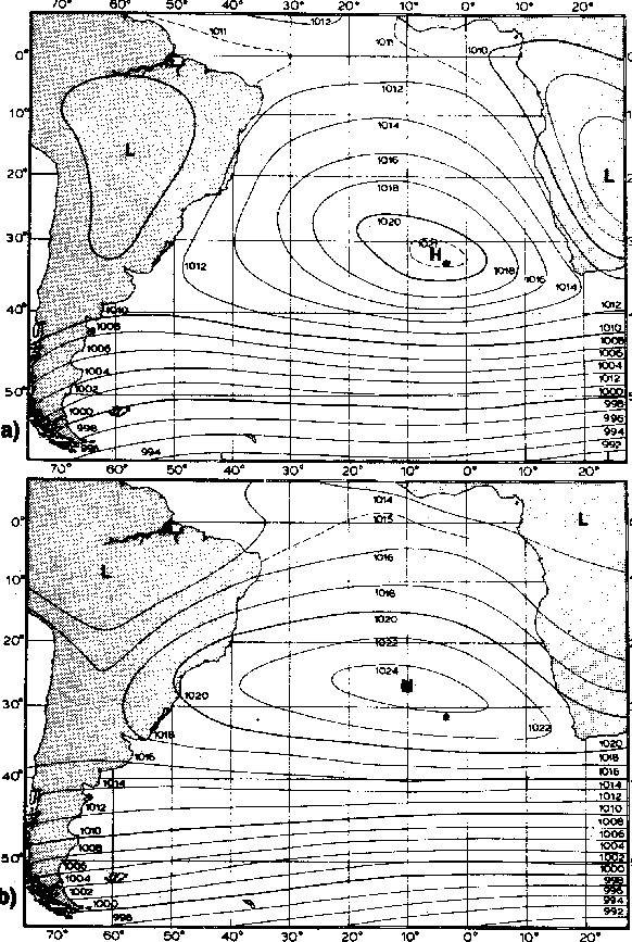 |
The wind field in the Benguela is mainly controlled by the South Atlantic high
pressure system (figure 1.6). This anticyclone oscillates seasonally
along a North-West (austral fall) / South-East (austral spring) axis. It
generates equatorward, upwelling favorable wind stress all around the year in
the Northern Benguela and mostly in summer in the Southern Benguela. The flow
is steered equatorward along the coast by a thermal barrier set-up by the
desert in the North and by the mountain range along the Cape Peninsula in the
South. In winter, the Southern Benguela system is under the control of westerly
moving depressions that travel past the southern tip of Africa, the dominant
winds being more North-Westerly [Shillington, 1998]. The upwelling season in the
Southern Benguela occurs between September to March. The along shore wind
maximum is situated offshore, inducing a cyclonic wind stress curl along the
coast [Shannon and Nelson, 1996].
Figure 1.7:
Cyclic weather pattern over the Benguela system, typical of summer
conditions. (a) South Atlantic high established - coastal low at Lüderitz -
southerly winds at Cape Town. (b) South Atlantic High ridging - gale force
winds at Cape Town - coastal low moves south. (c) South Atlantic High weakens -
North West winds at Cape Town, following the passage of the coastal low. (d)
South Atlantic High strengthens - southerly winds along the west coast. (e)
Berg wind conditions. Adapted from Nelson and Hutchings [1983].
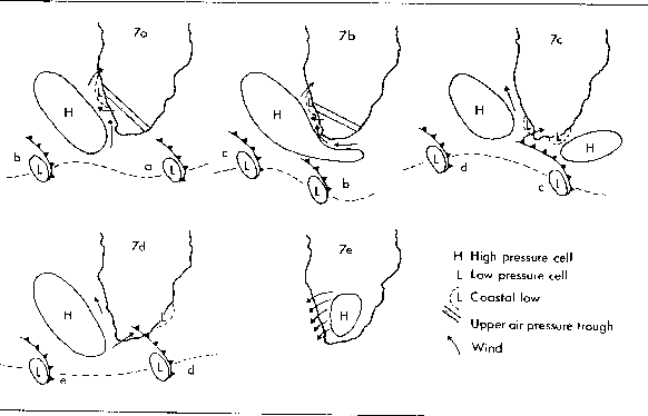 |
Low pressure cells propagate freely south of the African Continent over a
typical period of 1 to 2 weeks. Coastal cells of low pressure develop in
association with the approach of the cyclonic systems. These features,
named coastal lows, form near Lüderitz and travel South around the continent
as coastal trapped waves [Nelson and Hutchings, 1983]. Sometimes, a flow of dry
adiabatically heated air blows of the western escarpment when high pressure
cells form over the subcontinent: the so called "berg" winds [Shannon and Nelson, 1996]. The
typical cyclic summer weather pattern is portrayed on figure (1.7).
It has been proposed that this cycle induces a strong variability in coastal
upwelling and shelf currents of a period of 3 to 6 days [Nelson and Hutchings, 1983]. Pulsing
of the Benguela ecosystem has been related to the resonance between shelf waves
and the passage of coastal lows [Jury et al., 1990] and an optimum resonant pulse
interval of 10 days has been suggested [Jury and Brundrit, 1992]. Strong diurnal rotary
winds induced by land-sea breezes occur north of Cape Columbine [Shannon and Nelson, 1996].
Numerous studies have been conducted on local wind structures with the aim
of relating them to mesoscale structures observed in the Benguela upwelling system
[Jury, 1985a,Jury, 1985b,Jury et al., 1985,Jury, 1986,Jury, 1988,Kamstra, 1985,Taunton-Clark, 1985]. Areas of cyclonic wind
stress curl have been identified. They are induced by land topography in the
lee of Cape Columbine (i. e. in St. Helena Bay) and in the lee of Cape
Peninsula or by locally intensified atmospheric thermal front between
warm land and cool sea along the Namaqualand coastline ( S) [Jury, 1988].
The cyclonic wind stress curl induced by the wake in the lee of Cape Columbine
has been measured during typical events for the vertical atmospheric structure
[Jury, 1985a]. The wake (and then the cyclonic curl) is stronger in shallow
events (low inversion layer) than in deep events (high inversion layer). The
presence of upwelling plumes in the lee of Cape Peninsula and Cape Columbine
has been related to those topographically induced cyclonic wind stress curls
[Jury, 1985a,Jury, 1985b,Jury et al., 1985,Jury, 1986,Jury and Taunton-Clark, 1986,Jury, 1988,Kamstra, 1985,Taunton-Clark, 1985]. However, a
complete dynamical demonstration of the plume / wind stress curl relationship
is missing. In the same way, the presence of cyclonic eddies in the vicinity
of Cape Peninsula has been related to mesoscale temporal and spatial variations
in surface winds [Jury et al., 1985], but the formation of these eddies does not
appear to be correlated to local winds [Lutjeharms and Matthysen, 1995].
4 Along the West Coast
The wind induced coastal upwelling is characterized by a pronounced negative
sea surface temperature anomaly found mainly within the 150-200 km off the
West Coast of southern Africa [Shannon, 1985,Lutjeharms and Stockton, 1987]. Four major semi-permanent
upwelling centers are present in the Southern Benguela: the Lüderitz cell at
 S, the Namaqualand cell at around S, the Cape Columbine upwelling
plume at
S, the Namaqualand cell at around S, the Cape Columbine upwelling
plume at  S and the Cape Peninsula upwelling plume at S. The
presence of these cells has been related to local maximums in wind stress
curl [Jury, 1988], change in coastline orientation [Shannon and Nelson, 1996] or narrowing of
the shelf [Nelson and Hutchings, 1983]. The upwelled water originates from 200-300 m
[Nelson and Hutchings, 1983]. It is separated all along the coast from the offshore warmer
water by a well developed oceanic front [Brundrit, 1981]. Although highly
convoluted and variable, the front coincides approximately with the shelf
break. It shows large scale stationary features that have been related to the
existence of propagating barotropic shelf waves, although the latter
cannot explain
the standing nature of the process [Shannon, 1985].
S and the Cape Peninsula upwelling plume at S. The
presence of these cells has been related to local maximums in wind stress
curl [Jury, 1988], change in coastline orientation [Shannon and Nelson, 1996] or narrowing of
the shelf [Nelson and Hutchings, 1983]. The upwelled water originates from 200-300 m
[Nelson and Hutchings, 1983]. It is separated all along the coast from the offshore warmer
water by a well developed oceanic front [Brundrit, 1981]. Although highly
convoluted and variable, the front coincides approximately with the shelf
break. It shows large scale stationary features that have been related to the
existence of propagating barotropic shelf waves, although the latter
cannot explain
the standing nature of the process [Shannon, 1985].
2 Circulation
Figure 1.8:
Schematic flow-field of near-surface currents based on ADCP data
collected between November 1989 and January 1992. Velocity ranges indicated are
typical values. Adapted from Boyd and Shillington [1994].
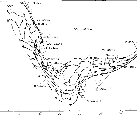 |
A strong equatorward surface baroclinic jet is in geostrophic balance with the
upwelling front
[Shillington, 1998] and follows the 200-300 m isobath [Nelson and Hutchings, 1983].
The speed of this semi-permanent jet ranges from 40 cm.s to 80
cm.s west of Cape Town [Boyd and Nelson, 1998] and is typically in excess of 50
cm.s offshore of Cape Columbine (figure 1.8) [Nelson and Hutchings, 1983]. It
can be strengthened near Cape Peninsula by the vicinity of Agulhas waters
with high steric height offshore [Strub et al. 1998]. Its width has been estimated at
some 20-30 km [Nelson and Hutchings, 1983]. As represented on figure (1.8), this jet
separates in two branches just north of Cape Columbine, one branch bending into
St. Helena Bay, the other, with a stronger intensity, flowing offshore.
Altimeter data show a convoluted equatorward jet several hundred kilometers
offshore North of S [Strub et al. 1998].
A net subsurface poleward flow, with averaged velocities of 4.5 cm.s to
6 cm.s, has been observed close to the shore along the entire west
coast [Boyd and Oberholster, 1994,Nelson, 1989]. It exhibits a wave-like motion with
periodicities of approximately three days. The cause of this flow along the
inner shelf is still unknown [Nelson, 1989].
Another characteristic feature of the Benguela system is the existence of the shelf
edge poleward undercurrent [Nelson and Hutchings, 1983]. It has been directly observed in a
number of cross sections and an average speed of 5-6 cm.s is given
[Shannon and Nelson, 1996]. It is part of a more extensive poleward motion stretching from the
coast across the bottom of the shelf to the Cape Basin [Nelson, 1989]. The
observation of oxygen-deficient water coming from a source area off Angola
along the shelf edge and onto the the shelf is another confirmation of the
existence of the poleward undercurrent [Dingle and Nelson, 1993]. Recent current
measurements
off Cape Columbine have revealed a deep poleward undercurrent of 11 cm.s
in autumn, 6.8 cm.s in winter, 7.4 cm.s in spring and 8.3
cm.s in summer [Nelson et al., 1999].
The averaged bottom temperature shows a cross-isobath trend on the shelf and
numerous hot-spots on coastal locations. It exhibits a flooded area North of
Cape Columbine, where the  C isotherm intrudes onto the shelf. On the
shelf, the bottom mixed layer has seldom a thickness less than 3 of the
total depth and it can be 2 or 3 times thicker on the shelf edge [Dingle and Nelson, 1993].
Tides along the West Coast are semi-diurnal, with a maximum spring range of about 2
m. The phase arrives almost almost simultaneously everywhere along the West
Coast. Tides induces small oscillations in the current in the order of 10-15
cm.s [Shillington, 1998].
The most impressive aspect of the Benguela system, and surely of the most
importance either from both a physical or a biological point of view, is the
high mesoscale activity that develops all along the coast. Four classes of
characteristic mesoscale features have been extracted from satellite images
of sea surface temperature [Lutjeharms and Stockton, 1987]: upwelling plumes, upwelling
filaments, upwelling eddies and Agulhas current filaments. The impact of
mesoscale activity on primary production in the Southern Benguela has been
illustrated by satellite imagery [Shannon et al., 1985]. Mesoscale activity can also
affect the transport pattern of fish larvae [Lutjeharms and Stockton, 1987]. The Agulhas
rings that have been described in section 1.2 might interfere
sporadically with the Benguela system.
C isotherm intrudes onto the shelf. On the
shelf, the bottom mixed layer has seldom a thickness less than 3 of the
total depth and it can be 2 or 3 times thicker on the shelf edge [Dingle and Nelson, 1993].
Tides along the West Coast are semi-diurnal, with a maximum spring range of about 2
m. The phase arrives almost almost simultaneously everywhere along the West
Coast. Tides induces small oscillations in the current in the order of 10-15
cm.s [Shillington, 1998].
The most impressive aspect of the Benguela system, and surely of the most
importance either from both a physical or a biological point of view, is the
high mesoscale activity that develops all along the coast. Four classes of
characteristic mesoscale features have been extracted from satellite images
of sea surface temperature [Lutjeharms and Stockton, 1987]: upwelling plumes, upwelling
filaments, upwelling eddies and Agulhas current filaments. The impact of
mesoscale activity on primary production in the Southern Benguela has been
illustrated by satellite imagery [Shannon et al., 1985]. Mesoscale activity can also
affect the transport pattern of fish larvae [Lutjeharms and Stockton, 1987]. The Agulhas
rings that have been described in section 1.2 might interfere
sporadically with the Benguela system.
Figure 1.9:
A schematic sea surface temperature ( C) map of a typical
developed Cape Peninsula upwelling tongue. Adapted from Taunton-Clark [1985].
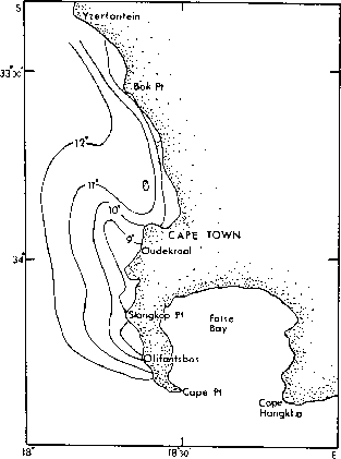 |
Figure 1.10:
Sea surface temperature ( C) distribution in St Helena Bay for 1
November 1980. An upwelling plume extends from Cape Columbine. Adapted from
Jury [1985a].
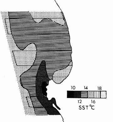 |
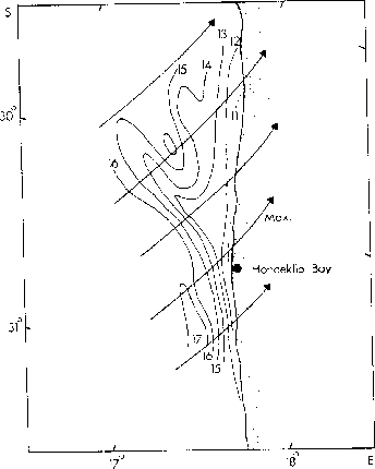
Figure 1.11:
Namaqualand sea surface temperature ( C) and wind
streamlines for 25 November 1980 (Max. = area of highest speed). The
Namaqualand upwelling plume develops from the coast. Adapted from Jury and
Taunton-Clark [1986].
 |
Upwelling plumes are variable, semi-permanent tongues of cold
water spreading from the major upwelling centers. Four sites of generation off
upwelling plumes have been recognized in the Benguela: Cape Peninsula, Cape
Columbine, Hondeklip Bay-Namaqualand and Lüderitz. The Cape Peninsula
upwelling plume is present during the summer months [Taunton-Clark, 1985], whereas it
can be masked during Northerly winds. It shows an elongated shape extending
north-westward (figure 1.9) enclosing cooler water at the
coast. The funneling of cold water through a canyon in the south-west (the Cape
Point Valley) [Shannon et al., 1981] and the influence of the coastal mountains on local
winds [Jury, 1988] has been advanced has explanations of the presence of this
plume. A similar tongue of cold water has been observed extending from
Cape Columbine (figure 1.10) [Shannon, 1985,Jury, 1985a,Jury, 1985b].
It has an inverted "S" characteristic shape,
suggesting topographic control [Shannon, 1985]. Whereas upwelling in Namaqualand
is confined into a coastal strip, a broad plume of cold water extends offshore
near S (figure 1.11). The base of this plume coincides
with a maximum in along shore winds and a broadening in the continental shelf
[Jury and Taunton-Clark, 1986]. The Lüderitz plume doesn't grow from a fixed location on the
coastline, but as it develops, it makes roughly always the same angle with the
coast [Lutjeharms and Stockton, 1987].
In comparison with upwelling plumes, upwelling filaments are narrower, not
standing, and short-lived features (between five days and five weeks)
extending from the upwelling front
[Lutjeharms and Stockton, 1987]. An in-situ investigation off a
filament have shown that it is a relatively shallow feature that is confined
in the upper 50 m. Filaments have typical elongations of 200 km [Shannon and Nelson, 1996],
ranging from 50 km to 600 km [Lutjeharms and Stockton, 1987]. In extreme cases, they may extend
1000 km or more offshore [Lutjeharms et al., 1991]. On average, two times more filaments
develop from Lüderitz than from the Cape Peninsula [Lutjeharms and Stockton, 1987]. ADCP
measurements have revealed the interaction between eddies and filaments North
of the Cape Peninsula [Nelson et al., 1999].
Figure 1.12:
Location of frontal eddies on the upwelling front from (a) February
1985, (b) August 1985 and (c) the whole of 1985, according to imagery from
NOAA-9 satellite. Adapted from Lutjeharms and Stockton [1987].
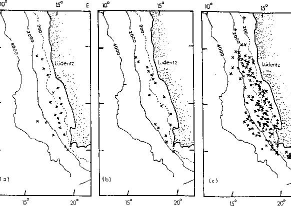 |
Eddies are numerous in the system with a preponderance
off-shore and downstream of the four major upwelling centers (figure
1.12). Their distributions show no clear seasonal patterns
[Lutjeharms and Stockton, 1987]. The Cape Peninsula has been recognized as a highly productive
area of cyclonic eddies with averaged diameters of 42 km  16 km. No
correlation exists between the formation of these eddies and the local winds
[Lutjeharms and Matthysen, 1995]. Vortex dipoles composed of eddies of about 50 km diameter has
been observed near Cape Columbine and Lüderitz [Stockton and Lutjeharms, 1988]. Altimeter data
has revealed the generation of cyclonic eddies from the coast and their
propagation offshore to the west [Strub et al. 1998].
One possible link between the Agulhas and the Benguela systems is the spreading
of long streak of warm water from the Agulhas current along the western edge of
the Agulhas Bank: the Agulhas filaments. They can interact with the Cape
Peninsula upwelling front and catalyse eddy formation from the cape
[Lutjeharms and Stockton, 1987] or increase steric height gradient at the front [Strub et al. 1998].
Intrusion of Agulhas water within 30 km of Cape Peninsula, flowing
northward at around 40-60 cm.s has been regularly observed [Boyd and Nelson, 1998].
Most of the Agulhas filaments detach from the Agulhas Current just downstream
of the southern tip of the Agulhas Bank. Six or seven are formed per year, each
usually lasting 3-4 weeks. Their average width is around 50 16 km and
their average length 530 166 km. They do not appear to extend
deeper than 85 m, but they can be responsible of between 5 and 15 of
the total interbasin salt flux generated by the Agulhas Current [Lutjeharms and Cooper, 1996].
16 km. No
correlation exists between the formation of these eddies and the local winds
[Lutjeharms and Matthysen, 1995]. Vortex dipoles composed of eddies of about 50 km diameter has
been observed near Cape Columbine and Lüderitz [Stockton and Lutjeharms, 1988]. Altimeter data
has revealed the generation of cyclonic eddies from the coast and their
propagation offshore to the west [Strub et al. 1998].
One possible link between the Agulhas and the Benguela systems is the spreading
of long streak of warm water from the Agulhas current along the western edge of
the Agulhas Bank: the Agulhas filaments. They can interact with the Cape
Peninsula upwelling front and catalyse eddy formation from the cape
[Lutjeharms and Stockton, 1987] or increase steric height gradient at the front [Strub et al. 1998].
Intrusion of Agulhas water within 30 km of Cape Peninsula, flowing
northward at around 40-60 cm.s has been regularly observed [Boyd and Nelson, 1998].
Most of the Agulhas filaments detach from the Agulhas Current just downstream
of the southern tip of the Agulhas Bank. Six or seven are formed per year, each
usually lasting 3-4 weeks. Their average width is around 50 16 km and
their average length 530 166 km. They do not appear to extend
deeper than 85 m, but they can be responsible of between 5 and 15 of
the total interbasin salt flux generated by the Agulhas Current [Lutjeharms and Cooper, 1996].
4 The nursery ground of the West Coast: St Helena Bay
St Helena bay can be defined in a broad sense as the wide shelf area
extending 200 km North of Cape Columbine (figure
1.3). South of Cape Columbine, the width of the shelf is narrow
(50 km) and becomes broader further north (up to 150 km).
The size repartition of anchovy larvae have shown that the area North of Cape
Columbine is the major nursery ground of the West Coast, with large numbers of
small anchovy larvae being advected into the area from the South [Boyd and Hewitson, 1983].
High concentrations of juvenile fish have been observed in the area [Hutchings, 1992].
Figure 1.13:
Schematic representation of currents in the Cape Columbine-St Helena
Bay area. Adapted from Shannon [1985].
 |
The Cape Columbine upwelling plume develops during upwelling events. Kamstra
[1985] and Jury [1985a] have related the generation of the
plume to the cyclonic wind stress curl in the vicinity of Cape Columbine. This
curl is generated by topographic effects on wind around the cape and it appears
to be pronounced during "shallow southeasterly events" (marine layer
thickness comparable to land elevation). Using radio tracked drifters, Holden
[1985] shows that whereas the flow is predominantly northward and
perturbed by small eddies, a cyclonic vortex remains in St. Helena Bay.
It connects to a southward current flowing along the coast (figure 1.13).
ADCP measurments show the same pattern in St Helena Bay with an inshore
curvature of the surface currents, bounding a broad area of weak mean currents
[Boyd and Oberholster, 1994]. Whereas stratification might be
important in the bay [Bailey and Chapman, 1985], current meter moorings near Cape Columbine
[Lamberth and Nelson, 1987] have demonstrated the transient barotropic nature of the flow.
Offshore and associated with a subsurface front, the baroclinic jet described
in section (1.4.2) follows the shelf edge with estimated surface
velocities of 60 cm.s (figure 1.13) [Shannon, 1985].
The Agulhas Bank forms the southernmost extremity of the African continent. It
is a wide triangular shelf extending up to 230 km south from the coast (figure
1.3). It has been recognized as the main spawning area for
sardines and anchovies in the Southern Benguela. The transport of eggs and
larvae between the western part of the Bank and the nursery grounds of the West
Coast is a major factor for the success of sardines and anchovies recruitment
[Fowler and Boyd, 1998].
The coastal boundary of the Agulhas Bank is forced by the wind. Easterly winds
can drive episodic coastal upwelling in summer. Inshore of the 100 m isobath,
the currents are weak and/or variable in speed and direction, with a net
North-West flow West of Cape Agulhas. This convergent North-West current system
funnels into the shelf edge jet of Cape Peninsula [Boyd and Oberholster, 1994], it is supposed
to be the path followed by the larvae to reach the West Coast [Fowler and Boyd, 1998].
Within the Bank, the summer vertical structure shows a strong stratification,
whereas it is well mixed in winter due to erosion by winter storms. Coastal
sea level and coastal current reversals reveal the passage of eastward
traveling coastal trapped waves [Boyd and Shilligton, 1994].
The eastern and offshore part of the Agulhas Bank is highly influenced by the
Agulhas current. It flows along the shelf edge, developing meanders, shear edge
features, borders eddies and reverse plumes on the Bank [Lutjeharms et al., 1989]. A ridge
of cool water surrounded by a cyclonic circulation has been observed from the
eastern to the central Bank [Boyd and Shilligton, 1994]. Vertical cross sections have shown
that uplift of cold water can be associated with reverse plumes and border
eddies [Lutjeharms et al., 1989]. There is not yet an explanation on how this feature is
formed [Boyd and Shilligton, 1994].
Typical currents spectra on the Benguela shelf show significant
peaks between 2.5 and 4 days [Nelson, 1989]. This have been related to
modulations in atmospheric forcing [Jury, 1986] or the passing of coastal
trapped waves [Shillington, 1998]. Jury and Brundrit [1992] have suggested a resonant
optimum pulse between oceanic and atmospheric coastal trapped waves of 10
days. Pulsing in the upwelling cycle has been found to range between 10 days
and more than 20 days [Jury et al., 1990]. A spectral analysis of tide gauge
measurements in Cape Town has exhibited a wide peak at around 10-15 days
[Schumann and Brink, 1990].
At the seasonal scale, upwelling is less variable in the Northern Benguela than
in the South where it stops during winter. Garzoli and Gordon [1996]
have found the strongest seasonal pattern in transport near the shelf edge at
S.
The system shows definite interannual variability with the occurrence of cold
and warm events [Shannon and Nelson, 1996]. The possibility of high sea-level events
propagating poleward from the equatorial Atlantic in the manner of the Pacific
El Niño has been confirmed [Brundrit et al., 1987]. Less intense and less frequent than
Pacific El Niño, the warm Benguela Niños events are characterized by the
advection of tropical water southwards along the coast of Namibia [Shannon and Nelson, 1996].
Benguela Niños are not necessarily in phase with the El Niño Southern
Oscillation.
The Benguela current differs from the other eastern boundary
systems by the poleward limitation of the coastal boundary at S. This
allows the South Indian western boundary current to approach closely and to
interact with the system. The dominant equatorward wind regime induces a strong
coastal upwelling separated from the open ocean by a well developed oceanic
front. This front is highly convoluted and follows roughly the shelf edge. It
is associated with a strong surface baroclinic jet that is present from Cape
Peninsula to Cape Columbine. After dividing near Cape Columbine, the outer
branch of the jet is found further offshore northward. Whereas the wind forcing
is mainly equatorward, poleward motion occurs in the Benguela in the form
of a poleward coastal counter current, a poleward undercurrent and a deep
poleward motion at the base of the shelf edge. High mesoscale activity is a
major characteristic of the system. It includes localized upwelling plumes,
upwelling filaments extending sometimes far offshore from the front, upwelling
eddies that can carry coastal products offshore in the ocean, Agulhas filaments
that sometimes interact with the upwelling front, coastal trapped waves, and
the famous Agulhas rings that are shed from the Agulhas Current. This
variability is exhibited on spatial scales ranging from around ten kilometers
to hundreds of kilometers and temporal scales ranging from a few days to
several months.
Sardines and anchovies have adapted their life strategy to the complexity and
peculiarities of the system by spawning on the Agulhas Bank, upstream of the
upwelling centers. St Helena bay, in the lee of Cape Columbine and hundreds of
kilometers away from the spawning grounds, appears to be the most important
nursery ground of the South African West Coast.
The Benguela has been extensively studied, but the complexity of the system is
such that numerous questions are still open. I would like to present
here a few that seem to be relevant for this manuscript:
- What is specific in the dynamics of St Helena Bay that make it a successful
nursery ground ?
- How does the transport work from the Agulhas Bank to the
upwelling centers ?
- What is the impact of mesoscale activity on the transport patterns?
There are several ways to explore these questions. During the last 30 years, a
large quantity of data has been collected, providing numerous insights
regarding the dynamics of the Benguela upwelling system. More data and new
oceanographic cruises could be set up to answer the questions listed to the
previous paragraph. However, numerical tools are now widely available and
become more and more relevant to explore coastal processes. In the Benguela,
modeling is in its infancy and we have taken the opportunity to explore the
dynamics of the system using an approach, as well as tools, that have never been
used in the region.
2 Recirculation and retention on the shelf in St. Helena
Bay
In this chapter, we will concentrate on the first question listed in the
summary of the first chapter: "Why is St. Helena Bay such a successful nursery
ground ?". The shelf being large in St. Helena Bay, idealised barotropic
numerical
experiments are conducted in order to explore the interactions between an
equatorward, upwelling favorable, wind forced current and the topogaphy of the
Bay.
Diagnostic analysis and analytical calculations bring to light the dynamics involved
in the simulations. The impact of the circulation on the retention of
biological
material in the Bay is explored through a tracer marking the age of the water
masses.
Dans ce chapitre, nous nous concentrerons sur la première question
énoncée dans le résumé du chapitre pr'ecédent:
"Quelle est la cause du succès de la nourricerie de la Baie de Ste Hélène ?".
La Baie de Ste Hélène présentant un large plateau, des expériences
idéalisées barotropes sont mises en place afin d'explorer les interactions
entre un courant vers l'équateur, forcé par un vent favorable a l'upwelling,
et la topographie de la baie. Des analyses diagnostiques, et des calculs analytiques
éclairent la dynamique impliquée durant les simulations.
L'impact de la circulation sur la rétention des composantes biologiques est
quantifiée à l'aide d'un traceur représentant l'age des masses d'eau.
The upwelling of the West Coast of South Africa provides the necessary
enrichment for the recruitment. But the driving mechanism of
coastal upwelling, the offshore Ekman transport, at the same time, advects the
larvae away from the productive area. Hence, the success of recruitment
requires the presence of a retention process that keeps the larvae in the
favorable area [Bakun, 1998]. If enrichment by upwelling occurs all along the
West Coast, the success of St. Helena Bay should be related to presence of
retention in the bay.
St. Helena Bay is located just North of Cape Columbine, one the two major capes
of the West Coast. It can be seen as a step-like indentation of 100 km in the
coastline. Associated with this topographic feature, the shelf broadens
dramatically, to reach a width of 150 km (figure 1.3). This
topographic configuration should alter the coastal circulation in a favorable
way for the recruitment.
To test this last statement, 2 hypotheses are assumed. Firstly, on a broad
relatively flat shelf like St. Helena Bay, following the criterion of Clark
and Brink [1985], baroclinic processes should be of less importance than
barotropic dynamics. Secondly, spatial and temporal wind variations, although
important, should not be necessary to produce a favorable environment during
upwelling events.
Following these hypotheses, a set of idealized numerical experiments are
undertaken to explore the influence of a cape and a broadening shelf on the
retention during the upwelling season (e. g. for a coastal circulation forced
by an equatorward wind).
The outline of this chapter is as follow. After a review of the interaction
between coastal currents and capes, a description of the numerical model is
provided. An analytical model of the barotropic processes gives characteristic
values for velocities and free surface elevation. Outputs of a reference
numerical experiment are analyzed and sensitivity tests are conducted, using a
range of values for wind forcing, bottom friction or different size of
capes. Different mechanisms, such as control by bottom friction or the
generation of standing waves, are tested to explain the flow patterns observed
in the experiments. Finally, a tracer showing the age of the water is
integrated into the model to quantify retention.
Interactions between capes and coastal currents are complex and remain
poorly understood; although they have been studied in many ways. Crepon et al.
[1984] solved analytically a linear upwelling two-layer model
around a rectangular promontory. Baroclinic and barotropic Kelvin waves
generated at the corner of the cape propagate poleward and can lead to
upwelling fluctuations independent of local winds. Further, they relate the
poleward undercurrent to the difference of the phase speeds between baroclinic
and barotropic waves. They found numerically the same pattern with different
shapes of cape. Batteen [1997] explains the enhancement of upwelling
equatorward of capes by conservation of potential vorticity in equatorward
flows. Downstream and inshore of the plume of upwelled water, an "upwelling
shadow" can be found such as that described by Graham and Largier [1997] for
Northern Monterey Bay where warm water is trapped at the coast behind a narrow
oceanic front.
Several laboratory experiments involved flow past capes. Davies et al. [1990]
introduced stratification in the case of a flat bottom and no rotation. Whereas
stratification determines all aspects of eddy generation or eddy shedding from
the capes, bottom friction seems to be crucial during the decay of the eddy
[Davies et al., 1990]. By introducing a counterclockwise rotation, Boyer and Tao
[1987a] showed that the response of the flow differs dramatically if the
cape is on the left or on the right looking downstream in the Northern
hemisphere. Their setting corresponds to respectively an equatorward and
poleward flow along an oceanic Eastern boundary. The poleward current passes
through three regimes, depending on the Burger number
(
 ; where
  is the Brunt-Väisälä frequency,
 is the water depth,
  is the Coriolis parameter and
  a characteristic
length scale):
a characteristic
length scale):
- Small S: flow fully attached, no eddy generated;
- Medium S:
generation of an attached anticyclonic eddy;
- Larger S: shedding of
anticyclonic eddies.
For the equatorward current, there is no fully attached regime:
- Small S: generation of an attached cyclonic eddy (quickly formed but
subsequently spins down);
- Larger S: shedding of cyclonic eddies.
Boyer et al. [1987b] have performed the same kind of experiments
with an obstacle on the left or on right of the flow, but involving this time
an homogeneous fluid. They found a complex wake motion for a certain range of
Rossby and Ekman parameters, and again strong differences if the cape is on
the left or on the right. In the case "cape on the left", the vortex shedding
is more regular, but in both cases, eddies can merge into larger structures
that can be, depending of the parameters, attached, shed or advected
downstream. Klinger [1983] has tested the influence of the Rossby
and Ekman numbers on the formation of anticyclones on slopes, by concentrating
on a barotropic flow past a corner in a rotating tank (poleward flow along an
eastern boundary). In this case, whereas the gyre size is approximately
proportional to the Rossby number, it is not strongly influenced by bottom
friction.
Narimousa and Maxworthy [1989] have built a more realistic
laboratory model to interpret satellite observations of coastal upwelling.
This experiment shows the effects of ridges and capes on the generation of
standing waves, meanders, filaments and eddies. The capes produce cyclones
inshore and filaments offshore. These experimental results are in good
agreement with satellite images of sea surface temperature off the West Coast
of the North American continent.
To describe the patterns measured in the lee of islands, Wolanski et al. [1984]
have introduced an "Island wake parameter": P from an Ekman pumping model for
the control of wake eddies. This parameter can predict if friction dominates
the flow (P 1), if there is a stable wake (P1) or if there is
apparition of instabilities (P
1), if there is a stable wake (P1) or if there is
apparition of instabilities (P 1). This result has been found to be in good
agreement with the flow patterns derived from remotely sensed imagery by
Pattiaratchi et al. [1986], but has been in bad agreement when bottom
topography is complex.
Similar studies have been conducted using numerical models. Becker [1991]
built a numerical model of a viscous flow past a cylinder
in a rotating frame, when the Rossby (Ro) and the Ekman (Ek) numbers are
small. She has found two key parameters for the boundary layer separation:
1). This result has been found to be in good
agreement with the flow patterns derived from remotely sensed imagery by
Pattiaratchi et al. [1986], but has been in bad agreement when bottom
topography is complex.
Similar studies have been conducted using numerical models. Becker [1991]
built a numerical model of a viscous flow past a cylinder
in a rotating frame, when the Rossby (Ro) and the Ekman (Ek) numbers are
small. She has found two key parameters for the boundary layer separation:
 , which is an equivalent of the "Island wake
parameter" and
, which is an equivalent of the "Island wake
parameter" and  the boundary layer thickness. The flow starts to
detach when
the boundary layer thickness. The flow starts to
detach when  , and the bubble length increases linearly with
 and with decreasing . The generation and evolution of eddies
around headlands by a tidal flow have been studied analytically and numerically
by Signell and Geyer [1991]. In a boundary layer model, detachment
occurs because of bottom friction as soon as an adverse pressure gradient is
established. They found using a 2D numerical model that the extent of
vorticity is limited by the frictional length scale:
and with decreasing . The generation and evolution of eddies
around headlands by a tidal flow have been studied analytically and numerically
by Signell and Geyer [1991]. In a boundary layer model, detachment
occurs because of bottom friction as soon as an adverse pressure gradient is
established. They found using a 2D numerical model that the extent of
vorticity is limited by the frictional length scale:
 . In
a two layer realistic numerical model of Oregon coast, Peffley and O'Brien
[1975] showed that bottom topography overwhelms coastline irregularities in the
generation of mesoscale upwelling features. On the contrary, using a realistic
3D numerical model of the California upwelling system, Batteen [1997] found
that wind forcing and coastline irregularities are key mechanisms for the
generation of meanders, eddies, jets and filaments. She showed that capes
"anchor" filaments and generate cyclonic eddies. The process of generation and
control of a cyclonic eddy past Point Conception (California) has been studied
by Oey [1996]. In a one and a half layer, reduced-gravity model (infinite
bottom layer), equatorward wind forced currents generate a cyclonic eddy past
the cape by advection of vorticity at the corner. Viscosity and the Rossby
number control it. This eddy is found again in a 3D realistic model of the
Santa Barbara Channel. It seems to follow the same processes of formation,
although bottom topography and beta effect are shown to become important for
longer time period (
. In
a two layer realistic numerical model of Oregon coast, Peffley and O'Brien
[1975] showed that bottom topography overwhelms coastline irregularities in the
generation of mesoscale upwelling features. On the contrary, using a realistic
3D numerical model of the California upwelling system, Batteen [1997] found
that wind forcing and coastline irregularities are key mechanisms for the
generation of meanders, eddies, jets and filaments. She showed that capes
"anchor" filaments and generate cyclonic eddies. The process of generation and
control of a cyclonic eddy past Point Conception (California) has been studied
by Oey [1996]. In a one and a half layer, reduced-gravity model (infinite
bottom layer), equatorward wind forced currents generate a cyclonic eddy past
the cape by advection of vorticity at the corner. Viscosity and the Rossby
number control it. This eddy is found again in a 3D realistic model of the
Santa Barbara Channel. It seems to follow the same processes of formation,
although bottom topography and beta effect are shown to become important for
longer time period ( days).
A main discrepancy between our study and Oey's [1996] work is the width
of the shelf in St Helena Bay that extends from 50 km to 150 km, while the
extension of the shelf in front of Point Conception is limited to 20 km. The
presence of those shallow waters invalidate the use of a one layer and a half
reduced gravity model, and bottom effects should be important in the
generation and control of cyclonic eddies. It appears then that the presence
and the shape of the bottom topography should overwhelm the effects related to
stratification. To quantify this, the Brunt-Väisälä frequency has
been calculated using recent temperature and salinity measurements in St.
Helena Bay. It has a typical value of
days).
A main discrepancy between our study and Oey's [1996] work is the width
of the shelf in St Helena Bay that extends from 50 km to 150 km, while the
extension of the shelf in front of Point Conception is limited to 20 km. The
presence of those shallow waters invalidate the use of a one layer and a half
reduced gravity model, and bottom effects should be important in the
generation and control of cyclonic eddies. It appears then that the presence
and the shape of the bottom topography should overwhelm the effects related to
stratification. To quantify this, the Brunt-Väisälä frequency has
been calculated using recent temperature and salinity measurements in St.
Helena Bay. It has a typical value of
 . Whereas
stratification is significant, the gentle bottom slope of St. Helena Bay (slope
coefficient:
. Whereas
stratification is significant, the gentle bottom slope of St. Helena Bay (slope
coefficient:
 %) satisfies the dynamic criterion for
barotropic shelf water response [Clark and Brink, 1985]:
%) satisfies the dynamic criterion for
barotropic shelf water response [Clark and Brink, 1985]:
 ,
where is the Coriolis parameter. In St Helena Bay,
,
where is the Coriolis parameter. In St Helena Bay,
 . This 'bottom slope' Burger number allows us to state
that whereas density related processes such as upwelling and associated baroclinic
coastal jets might be important, the major characteristics of the circulation
can be described by barotropic dynamics. This is consistent with the barotropic
nature of the flow measured by Lamberth and Nelson [1987].
In this chapter, we will only concentrate on the barotropic response of a
coastal ocean to equatorward wind forcing. Baroclinic effects are expected
to be secondary or localized [Graham and Largier, 1997] and will be
investigated in future work. The aim of this chapter is to understand the
processes controlling the pattern of flow detachment and eddy generation in
the vicinity of Cape Columbine.
. This 'bottom slope' Burger number allows us to state
that whereas density related processes such as upwelling and associated baroclinic
coastal jets might be important, the major characteristics of the circulation
can be described by barotropic dynamics. This is consistent with the barotropic
nature of the flow measured by Lamberth and Nelson [1987].
In this chapter, we will only concentrate on the barotropic response of a
coastal ocean to equatorward wind forcing. Baroclinic effects are expected
to be secondary or localized [Graham and Largier, 1997] and will be
investigated in future work. The aim of this chapter is to understand the
processes controlling the pattern of flow detachment and eddy generation in
the vicinity of Cape Columbine.
2 Model description
The numerical code is the barotropic part of the SCRUM 3D oceanic model from
Rutgers University [Song and Haidvogel, 1994,Hedström, 1997]. The model is based on the hydrostatic
and Boussinesq approximations. The barotropic component solves the vertically
integrated momentum equation [Hedström, 1997] and in our case density variations
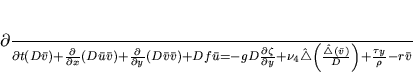
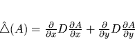
are not taken into account. SCRUM conserves the first moments of u and v. This
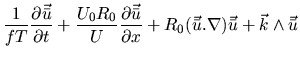
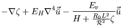
is accomplished by using the flux form of the momentum equations [Hedström, 1997]:
 |
(1) |
 |
(2) |
Where
 is the operator:
 |
(3) |
The continuity equation takes the from:
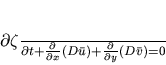 |
(4) |
Where:
- x is the along shore coordinate (positive towards the equator).
- y is the cross-shore coordinate (positive towards the open ocean).
 and
and  are the vertically
averaged flow velocity respectively in each coordinate direction.
are the vertically
averaged flow velocity respectively in each coordinate direction.
 is the free surface elevation.
 is the total water column depth,
  , where is the
ocean depth.
, where is the
ocean depth.
- is the Coriolis parameter,
 , where
 is the Earth angular velocity and
  is the latitude. In our
case, because the time scale O(10 days) and the length scales O(100 km) are
small enough, we can assume a constant Coriolis parameter as explained by
Kundu [1990].
is the latitude. In our
case, because the time scale O(10 days) and the length scales O(100 km) are
small enough, we can assume a constant Coriolis parameter as explained by
Kundu [1990].
 s at Cape Columbine.
 is the Earth gravity acceleration,
  m.s
m.s .
.
 is the lateral biharmonic constant mixing coefficient
(m
is the lateral biharmonic constant mixing coefficient
(m .s).
.s).
 is the linear bottom drag coefficient (m.s).
-
 and
and
 are the
kinematic surface momentum fluxes (wind stress) respectively in each
coordinate direction (m
are the
kinematic surface momentum fluxes (wind stress) respectively in each
coordinate direction (m .s).
.s).
In order to preserve the mesoscale structures, a bi-harmonic operator
parameterizes the horizontal viscosity. For the sake of simplicity and as
suggested by Csanady [1982], the weak tidal currents are not
resolved and the bottom stress is chosen to be proportional to the barotropic
velocities. The linear bottom friction coefficient is initially fixed at a
typical value found in the literature (
 m.s), but
sensitivity tests have been conducted to explore the strong impact of this
coefficient on the circulation.
m.s), but
sensitivity tests have been conducted to explore the strong impact of this
coefficient on the circulation.
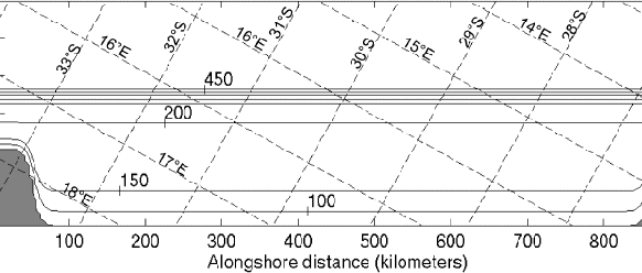
Figure 2.1:
The periodic analytical bathymetry implemented in the model.
 |
The regular grid has a 5 km resolution along shore and cross-shore. The
coastline is represented by a free-slip wall in x=0 and its variations are
modelized by masking the inshore grid points where the depth is less than 50 m
[Hedström, 1997]. The most straightforward way to close the domain
offshore and on the sides is the use of a periodical channel: a free-slip
wall far beyond the shelf break and all the outflows (inflows) at the southern
boundary being inflows (outflows) for the northern boundary. Those boundary
conditions allow an along shore wind forced circulation and conserve mass. The
presence of the shelf break should isolate the shelf circulation from the
effects of the offshore wall [Csanady, 1978]. The bottom topography is
represented by a set of analytical functions which retains the main
topographical features, thus focusing attention on the effects of Cape
Columbine and the widening shelf on the circulation. The bathymetry has
been made periodic to allow the use of the periodic channel (figure
2.1). Nevertheless, this topography is still comparable for the
first 300 km to the topography of St Helena Bay (see figure
1.3). The second cape on the right might perturb the solution
at distances up to 300 km (the external Rossby radius) upwind of the cape,
thus interfering with our area of interest. For this reason, the experiments
are run with an along shore domain of 900 km. The atmospheric forcing is a
constant wind stress parallel to the x-axis, accounting for the summer
southeaster wind. The wind stress is uniform in space and constant in time for
a given experiment. A set of runs with wind stress ranging from 0.02 N.m
to 0.2 N.m are performed to investigate the effects of the intensity of
the wind forcing.
To illustrate the basic mechanism for wind forcing in the coastal ocean, Brink
[1998] solved a linearized along shore wind forced model where the spatial
scales are small enough compared to the external Rossby radius of deformation
to neglect divergence, and where the along shore scales are large compared to
the cross-shore ones (boundary layer approximation, [Csanady, 1998]). This
implies that the along shore flows are much stronger than the cross-shelf ones
[Brink, 1998]. This is not true near Cape Columbine but it can be a good
approximation further North. Thus, the results from this model can give us a
scale for the mean along shore velocities and the sea surface slope to compare
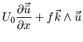
with the numerical experiment outputs. If the wind forcing is uniform,
the along shore variations can be neglected and the barotropic equations of
motion with linear bottom friction become [Brink, 1998,Csanady, 1998], using the same
notations as in the previous paragraph:
 |
(5) |
 |
(6) |
 |
(7) |
The along shore velocities are forced by the along shore wind and the free
surface remains in geostrophic equilibrium with the along shore velocities.
In order to satisfy equation (2.7) and the fact that there
is
no cross-shore
flow at the coastal boundary, the cross-shelf transport has to vanish
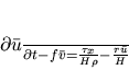
everywhere [Brink, 1998]. Starting from rest at t=0 with a constant wind
stress, we obtain from equation (2.5):
 |
(8) |
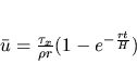
If the maximum depth is 500 m, the solution is nearly stationary after 40
days with along shore velocities:
 |
(9) |
This result shows that bottom friction allows us to expect for the numerical
experiments a steady solution after nearly 50 days with along shore
velocities of the order of magnitude:
 , resulting from
a balance between the wind stress and the bottom friction. For example if the
wind stress value equal 0.1 N.m, after 50 days the mean
along shore velocities should be
, resulting from
a balance between the wind stress and the bottom friction. For example if the
wind stress value equal 0.1 N.m, after 50 days the mean
along shore velocities should be  m.s.
m.s.
4 The reference experiment
For the reference experiment, the constant wind stress value is fixed at
 N.m corresponding to the average wind stress
measured in the area during upwelling seasons (
N.m corresponding to the average wind stress
measured in the area during upwelling seasons (
 N.m). The linear bottom friction coefficient value is r =
 m.s and the viscosity parameter is set to the lowest possible
value to avoid numerical noise (
m.s and the viscosity parameter is set to the lowest possible
value to avoid numerical noise (
 ms).
ms).
Figure 2.2:
Barotropic velocities and free surface elevation for the
reference experiment in the vicinity of Cape Columbine:
a) day 10 (maximum velocity: 62 cm.s, averaged velocity: 16
cm.s),
b) day 30 (maximum velocity: 69 cm.s, averaged velocity: 25
cm.s),
c) day 50 (maximum velocity: 70 cm.s, averaged velocity: 28
cm.s ),)
d) day 50 for the same experiment with no shelf-edge (maximum velocity: 71
cm.s, averaged velocity: 30 cm.s).
The horizontal coordinates are in kilometers and the greyscale range for the
free surface elevation is in centimeters. The interval between the isolines is
5 cm.
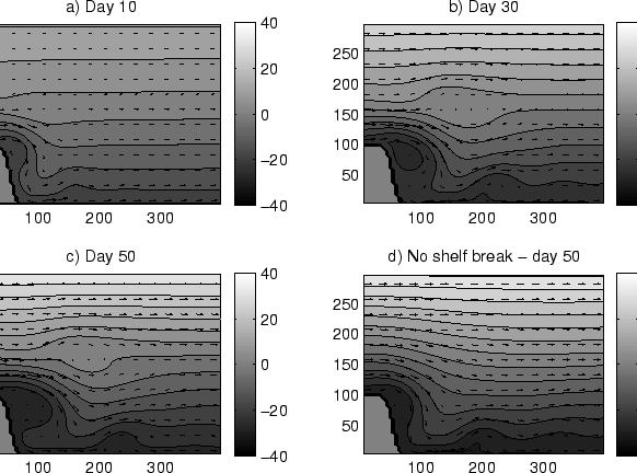 |
Starting from rest, an equatorward current develops in response to the
equatorward wind forcing. In balance with the along shore velocities, a cross
shelf slope of the free surface is set up (figures 2.2-a,
2.2-b and 2.2-c). The solution becomes steady after
50 days (figure 2.2-c), the average sea surface slope value is
between 0.17 and 0.38 centimeters per kilometer and the mean along shore
velocities are approximately equal to  m.s. Although the presence
of a coastline and bottom topography variations induces a drag that reduces the
along shore velocity, its value stays in the same order of magnitude as in the
analytical solution. Four scaling parameters allow us to compare the results
with other studies:
m.s. Although the presence
of a coastline and bottom topography variations induces a drag that reduces the
along shore velocity, its value stays in the same order of magnitude as in the
analytical solution. Four scaling parameters allow us to compare the results
with other studies:
- the Rossby number,
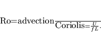 |
(10) |
- Because of the use of a biharmonic operator, the Reynolds number takes
the form:
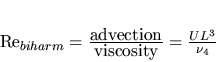 |
(11) |
- The Reynolds number associated with bottom friction,
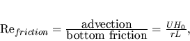 |
(12) |
which is equivalent to the 'island wake parameter' P introduced by Wolanski
et al. [1984]. A scaling analysis shows that it is equivalent to the
parameter defined by Becker [1991] (The same analysis shows that the
lateral boundary layer thickness defined by Becker [1991] is in our case:
 ).
).
- The Ekman number,
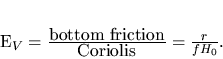 |
(13) |
Where,
- U is a characteristic velocity,
 m.s.
m.s.
- f is the Coriolis parameter,
 .
.
- L is a characteristic length scale, for example the size of the cape:
 km.
km.
- is the viscosity parameter,

 .
.
 is a characteristic depth,
  m on the shelf.
- is the bottom friction parameter,
 .
.
From these values we obtain:
 ,
,
 ,
,
 and
and
 . Hence, Coriolis acceleration and the resultant
pressure
gradient are the main driving forces and at the first order, advection and
bottom friction are the two important terms controlling the flow. Further,
those terms show that this experiment is in the attached-cyclonic-eddy regime
[small Rossby number, small Burger number (null in our case)] when the cape is
on the left (in the Northern Hemisphere) of the study of Boyer and Tao
[1987a].
. Hence, Coriolis acceleration and the resultant
pressure
gradient are the main driving forces and at the first order, advection and
bottom friction are the two important terms controlling the flow. Further,
those terms show that this experiment is in the attached-cyclonic-eddy regime
[small Rossby number, small Burger number (null in our case)] when the cape is
on the left (in the Northern Hemisphere) of the study of Boyer and Tao
[1987a].
 shows that this regime corresponds to the
stable wake regime of Wolanski et al. [1984a].
shows that this regime corresponds to the
stable wake regime of Wolanski et al. [1984a].  and
and
 are at the limit between the detachment and the
no-detachment regime of Becker [1991, see figure 7]. The small Rossby and Ekman
numbers correspond to the stable wake regime described by Boyer at al.
[1987b, see figure 3].
The reference experiment shows that the bottom topography associated with Cape
Columbine generates three main features:
are at the limit between the detachment and the
no-detachment regime of Becker [1991, see figure 7]. The small Rossby and Ekman
numbers correspond to the stable wake regime described by Boyer at al.
[1987b, see figure 3].
The reference experiment shows that the bottom topography associated with Cape
Columbine generates three main features:
- Attached cyclonic eddy: before day 10, the flow detaches from Cape
Columbine and generates an attached cyclonic eddy (figure 2.2-a,
x=50 km y=100 km). The size of the eddy is approximately 60 km at day 10 and
expands to a size of 110 km by day 50 (figures 2.2-b and
2.2-c). The presence of this stationary attached-cyclonic-eddy is
in agreement with the in-situ measurements of Holden [1985] and the recent
averaged ADCP data of Boyd and Oberlholster [1994]. It can be compared with
the schematic representation of the currents in St Helena Bay (figure
1.13) made by Shannon [1985]. This is also in agreement with the
experimental results of Boyer and Tao [1987a] for the cape on the left
(Northern Hemisphere), the smallest Burger number and
 . Further,
the presence of the cyclone and the strength of the velocities match the
results of the 3D model of Oey [1996, see figure 12 and figure 13]. In the
Santa Barbara Channel model, which includes baroclinic processes, Oey [1996]
applied an equatorward wind stress similar to the forcing of the reference
experiment. The bottom fiction is quadratic (
. Further,
the presence of the cyclone and the strength of the velocities match the
results of the 3D model of Oey [1996, see figure 12 and figure 13]. In the
Santa Barbara Channel model, which includes baroclinic processes, Oey [1996]
applied an equatorward wind stress similar to the forcing of the reference
experiment. The bottom fiction is quadratic (
 ) and the
grid resolution is 5/3 km. The equatorward flow associated with a pronounced
coastal upwelling is comparable with the barotropic velocities obtained here,
and forms a stationary cyclonic eddy in the lee of Point Conception. The size
of this eddy is approximately half the size of our barotropic eddy. This
discrepancy might be due to the depth of the shelf (300 m versus 150 m in our
experiment), the width of the shelf (50 km versus 150 km in our experiment) or
the presence of the Santa Barbara islands that might block the cyclone
extension.
) and the
grid resolution is 5/3 km. The equatorward flow associated with a pronounced
coastal upwelling is comparable with the barotropic velocities obtained here,
and forms a stationary cyclonic eddy in the lee of Point Conception. The size
of this eddy is approximately half the size of our barotropic eddy. This
discrepancy might be due to the depth of the shelf (300 m versus 150 m in our
experiment), the width of the shelf (50 km versus 150 km in our experiment) or
the presence of the Santa Barbara islands that might block the cyclone
extension.
- Influence of the shelf break: the steep shelf edge offshore (figure 2-b,
y=150 km) apply a strong topographic constraint on the flow, prohibiting
cross-topographic currents. Thus, mass conservation implies that the
velocities between Cape Columbine and the shelf break (figures 3-a, 3-b and
3-c, for x=0 km and y=0 to 150 km) are stronger than in the other parts of
the shelf. This can affect the detachment process. An experiment with no shelf
break (figure 2.2-d) shows that at day 50, the size of the
cyclonic eddy is approximately 60 the size of the eddy in the reference
experiment. The value of the along shore velocities near the tip of the cape is
80 the value of the velocities in the reference experiment. Further,
vortex squashing produces an anticyclonic bend on the shelf edge
(figure 2.2-c, x=180 km, y=150 km) and a divide in the currents
(figure 2.2-c, x=110 km, y=150 km). Its location corresponds
approximately to the location of the Columbine divide described by Shannon
[1985a], and it can be an explanation of this phenomenon.
- Upstream blocking: the artificial cape on the right seems to have no
influence on the detachment processes, but it produces weak near shore
velocities on the right of the shelf (figure not shown). This effect
can be felt up to 300 km [O(external Rossby radius of deformation)] upstream
of the cape. Because we use a large domain (900 km along shore), this phenomenon
does not affect our area of interest. This has been tested using a smaller
domain (600 km along shore) and the similarities between the solutions validate
the use of the periodic channel.
To understand the processes involved in the cyclone generation, the
dynamical terms have been computed from the model outputs using equations
(2.1) and (2.2). They have been rewritten in
the form of a sum of acceleration vectors as follow:
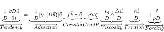 |
(14) |
Where  is the vertically averaged flow velocity,
 is the wind stress and
  is a vertical
unit vector. Because
is a vertical
unit vector. Because
 and
and
 , the
terms of equation (2.14) are respectively equivalent to the
terms of the vertically averaged momentum equation:
, the
terms of equation (2.14) are respectively equivalent to the
terms of the vertically averaged momentum equation:
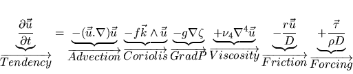 |
(15) |
Figure 2.3:
Accelerations (m.s) applied to the water particles for
the reference experiment at day 50 (the contours represent the free surface
elevation). a) At zero order, the balance between pressure
gradient and Coriolis acceleration dominates the dynamics. b) First order
tendency terms: by summing the pressure gradient and the Coriolis acceleration
vectors, the zero order balance can be filtered out and the first order terms
can be studied. Note that this terms are 20 times smaller than the zero order
ones.
 |
It appears (figure 2.3-a) that, at zero order, the balance between
pressure
gradient and Coriolis acceleration overwhelms the other accelerations. This is
in agreement with the small Rossby and Ekman numbers found previously. The
Coriolis acceleration pushes the flow offshore, creating an Ekman transport
away from the coast, in agreement with the upwelling models. Because of mass
conservation, this transport produces a down slope toward the coast in the
free surface, generating a pressure gradient in balance with the Coriolis
acceleration [Csanady, 1982].
By summing the pressure gradient and the Coriolis acceleration
vectors, we can filter out the zero order balance and get the
equilibrium at the first order [figure 2.3-b, note that these
accelerations
are 20 times smaller than in figure 2.3-a, in agreement with Ro and Ek
 ]. At this order, most of the terms start to be important. In the
following, we call the sum of the pressure gradient and the Coriolis
acceleration: the ageostrophic pressure gradient.
]. At this order, most of the terms start to be important. In the
following, we call the sum of the pressure gradient and the Coriolis
acceleration: the ageostrophic pressure gradient.
- Viscous terms are of an order of magnitude lower than the other ones.
They have some relative importance near the tip of the cape (figure
2.3-b,
x=40 km, y=100 km). As explained by Becker [1991], viscosity has to be small
for detachment to occur.
- Around the external part of the eddy (figure 2.3-b, x=50 to 130
km, y=70 to 130 km), there is a competition between advection and ageostrophic
pressure gradient. It appears that around the eddy (figure 2.3-b,
x=140 km, y=100 km), the radius of curvature of the flow is approximately
 km and the tangential velocities are about
  m.s. Then the
normal acceleration is
m.s. Then the
normal acceleration is
 m.s, which is close to the value of the advective acceleration
(
m.s, which is close to the value of the advective acceleration
(
 m.s). This shows a cyclo-geostrophic
equilibrium around the eddy. This advective acceleration, forcing the water
particles away from the cape, seems to be responsible for the detachment.
m.s). This shows a cyclo-geostrophic
equilibrium around the eddy. This advective acceleration, forcing the water
particles away from the cape, seems to be responsible for the detachment.
- Away from perturbations (figure 2.3-b, for example y220 km),
the wind forcing and bottom friction relative equilibrium controls the
along shore velocities as in the analytical solution.
- Another equilibrium occurs where the velocities are weak: inside the eddy
(figure 2.3-b, x=75 km, y=70 km) and in the upstream blocking area
(x=650 to 850 km, y=0 to 60 km, figure not shown). In those places, the
Coriolis acceleration is weak and a static wind stress-pressure gradient
balance prevails.
2 Vorticity balance
To refine the study, curls of the acceleration vector fields extracted from
equation (2.14) are computed to obtain the terms of the
equation
for the
vertically averaged vertical component of vorticity,  . Their physical
meaning can be illustrated by deriving the curl of equation
(2.15) and introducing the continuity equation
(2.4):
. Their physical
meaning can be illustrated by deriving the curl of equation
(2.15) and introducing the continuity equation
(2.4):
-
 is the advection
of vorticity added to the vortex stretching associated
with relative vorticity.
is the advection
of vorticity added to the vortex stretching associated
with relative vorticity.
-
 is the vortex
stretching associated with planetary vorticity. Because
the Rossby number is small, this term is much larger (10 to 100 times) than the
vortex stretching associated to relative vorticity.
is the vortex
stretching associated with planetary vorticity. Because
the Rossby number is small, this term is much larger (10 to 100 times) than the
vortex stretching associated to relative vorticity.
- As explained by Signell and Geyer [1991], the first term of
 is the vorticity dissipation by
bottom friction, and the second one is the 'slope torque' which acts as a
source of vorticity when there is a component of velocity normal to a depth
gradient. These two terms are in the same order of magnitude. Because
, the curl of bottom friction should be the same order
of magnitude as the advection of vorticity.
is the vorticity dissipation by
bottom friction, and the second one is the 'slope torque' which acts as a
source of vorticity when there is a component of velocity normal to a depth
gradient. These two terms are in the same order of magnitude. Because
, the curl of bottom friction should be the same order
of magnitude as the advection of vorticity.
- The first term of
 is the Ekman pumping associated with the wind stress curl and
the second term is, by analogy with the 'friction slope torque', a 'wind stress
slope torque' which can be a source of vorticity when the wind is normal to
a depth gradient. In our case, for
is the Ekman pumping associated with the wind stress curl and
the second term is, by analogy with the 'friction slope torque', a 'wind stress
slope torque' which can be a source of vorticity when the wind is normal to
a depth gradient. In our case, for  and
and 
 ,
the order of magnitude of the ratio between 'wind stress slope torque' and
advection of vorticity is:
,
the order of magnitude of the ratio between 'wind stress slope torque' and
advection of vorticity is:
 |
(17) |
This term can not be neglected. Its effects can be illustrated by traking
the curl of the analytical solution for the velocities (equation
2.8). During the spin-up, because is a function of y,
is also a function of y. Thus the vorticity is:
In this case, the vorticity produced continually from the beginning of the
experiment by the 'wind stress slope torque', is progressively dissipated by
bottom friction and 'friction slope torque'. Thus, after 50 days, the
stationary solution is irrotational. In the same manner as the 'friction slope
torque', the 'wind stress slope torque' appears because surface and bottom
stresses have a stronger effect in shallow waters than in deep waters.
Figure 2.4:
Tendency terms of the vorticity equation ( ), computed
from the dynamical terms at day 50 for the reference experiment: a) advection
of vorticity, b) curl of bottom friction, c) vortex stretching, d)
lateral viscous dissipation, e) wind stress slope torque, f) curl of the
pressure gradient. The horizontal coordinates are in kilometers and the
greyscale range represents the values in , multiplied by
), computed
from the dynamical terms at day 50 for the reference experiment: a) advection
of vorticity, b) curl of bottom friction, c) vortex stretching, d)
lateral viscous dissipation, e) wind stress slope torque, f) curl of the
pressure gradient. The horizontal coordinates are in kilometers and the
greyscale range represents the values in , multiplied by
 , except for the values of curl of the pressure gradient which are
multiplied by
, except for the values of curl of the pressure gradient which are
multiplied by  to show the validity of the computation.
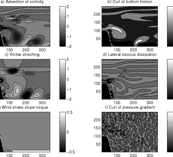 |
Figure (2.4) exhibits the relative importance of the vorticity
equation terms in
the vicinity of Cape Columbine. The advection of vorticity (figure
2.4-a)
contains as well the vortex stretching associated to relative vorticity, but
this term is one order of magnitude smaller than the other terms. The curl of
bottom friction (figure 2.4-b) contains both the bottom
dissipation
and the
'friction slope torque' and is thus not proportional to relative vorticity in
shallow waters. The vortex stretching (figure 2.4-c) is the
vortex stretching associated to planetary vorticity. The unit of these
terms is and
for clarity the values have been multiplied by  (figures
2.4-a, 2.4-b, 2.4-c,
2.4-d and 2.4-e). To validate the
approximations made in deriving the tendency terms, the curl of the pressure
gradient has been also portrayed, multiplied by
(figures
2.4-a, 2.4-b, 2.4-c,
2.4-d and 2.4-e). To validate the
approximations made in deriving the tendency terms, the curl of the pressure
gradient has been also portrayed, multiplied by  (figure
2.4-f).
We can then extract a number of equilibriums:
(figure
2.4-f).
We can then extract a number of equilibriums:
- The balance between advection of vorticity and vortex
stretching occurs almost everywhere where the slopes are strong: on the shelf break
(figures 2.4-a and 2.4-c, y=150 to 200 km) and
in the bay (figures 2.4-a and 2.4-c, y=0 to 60
km)
- Around the external part of the eddy, where the shelf is relatively flat
and the dynamics are cyclo-geostrophic (see previous section), the curl of
bottom friction balances the advection of vorticity (figures
2.4-a and 2.4-b, x=50 to 130 km, y=70 to 130
km). This balance seems to follow the contour of the eddy, and might control
its extension.
- As pointed out in the previous section, the
lateral viscosity has some importance near the tip of Cape Columbine. In figure
2.4-d, the viscous boundary layer is clearly seen for x=0 to 50
km and y=100 to 110 km. Past the cape, there is a detachment of this boundary
layer (figure 2.4-d, x=50 to 80 km, y=115 km).
- In shallow waters, the friction and wind stress slope torques start to
have a strong influence and seem to be in balance for x80 km and y=0 to 10
km (figures 2.4-b and 2.4-e).
We can expect from the second point that the size of the eddy is
controlled by the balance between advection of vorticity and curl of bottom
friction. From this, we can extract a characteristic length scale l:
 |
(19) |
 |
(20) |
This length scale can be seen as a frictional e-folding distance and is
equivalent to the eddy length scale  described by Pattiaratchi et al.
[1986] and Wolanski et al. [1984]. It is also equivalent to the frictional
length scale
described by Pattiaratchi et al.
[1986] and Wolanski et al. [1984]. It is also equivalent to the frictional
length scale  tested by Signell and Geyer [1991].
Taking the analytical result (equation 2.9) for the
characteristic velocities, the equation (2.20) becomes:
tested by Signell and Geyer [1991].
Taking the analytical result (equation 2.9) for the
characteristic velocities, the equation (2.20) becomes:
 |
(21) |
That gives us a characteristic eddy length scale which is a function of the
wind stress and of the linear bottom friction parameter. This length scale
can be compared to the size of the eddy. In this example, = 150 m,
 m.s, and
m.s
so
that
m.s, and
m.s
so
that
 km (the difference with the model outputs can be seen in figure
2.2).
To test the effects of the surface wind stress, the bottom friction
coefficient, the size of the cape, the grid resolution, the viscosity
coefficient and the domain size on the recirculation process, several numerical
experiments are conducted by varying one parameter at a time. Within realistic
parameter values, the grid resolution and the viscosity do not have much effect
on the cyclone generation. However, the nature of the cyclone does depend on
bottom friction, wind and the size of the cape.
Using the same parameters as in the reference experiment, ten experiments are
run with different along shore wind stress values, varying from
km (the difference with the model outputs can be seen in figure
2.2).
To test the effects of the surface wind stress, the bottom friction
coefficient, the size of the cape, the grid resolution, the viscosity
coefficient and the domain size on the recirculation process, several numerical
experiments are conducted by varying one parameter at a time. Within realistic
parameter values, the grid resolution and the viscosity do not have much effect
on the cyclone generation. However, the nature of the cyclone does depend on
bottom friction, wind and the size of the cape.
Using the same parameters as in the reference experiment, ten experiments are
run with different along shore wind stress values, varying from  N.m to
  N.m. These wind stress values correspond to wind
velocities at 10 m elevation of about
N.m. These wind stress values correspond to wind
velocities at 10 m elevation of about  m.s to
  m.s .
m.s .
Figure 2.5:
Barotropic velocities and sea surface elevation at day 100
for different values of the along shore wind stress. a) 0.05
(maximum velocity: 38 cm.s, averaged velocity: 12 cm.s), b) 0.15
N.m (maximum velocity: 100 cm.s, averaged velocity: 36
cm.s), c) 0.2 N.m (maximum velocity: 130 cm.s, averaged
velocity: 46 cm.s). The horizontal coordinates are in kilometers and the
greyscale range for the free surface elevation is in centimeters. The
interval between the isolines is 2 cm for (a), 6 cm for (b), and 8 cm for (c).
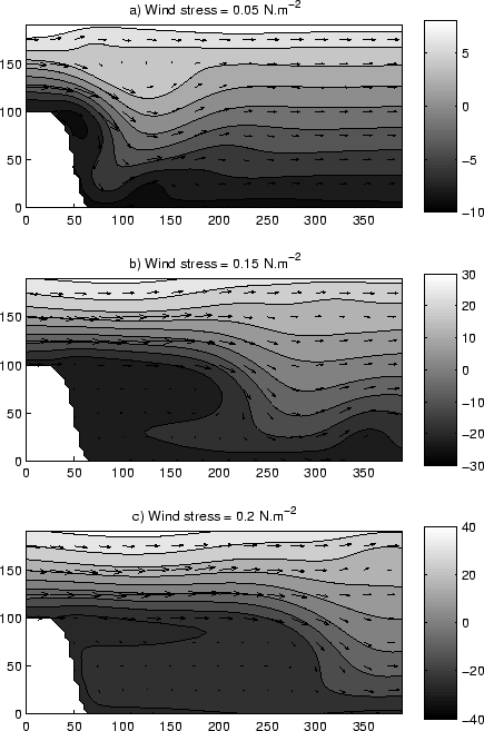 |
In all cases, the solution is steady after 50 days and the order of magnitude
of the mean velocities is in agreement with the analytical solution (figure
2.5). The characteristic velocities range from  m.s to
  m.s. The associate scaling parameters are,
using the same characteristic numbers as in section 2.4:
m.s. The associate scaling parameters are,
using the same characteristic numbers as in section 2.4:
-
 to
to

-
 to
to

-
 to
to 
-
as in the reference experiment.
This corresponds to the same regime as for the reference experiment: small Rossby
and Ekman numbers, large viscous Reynolds number and friction Reynolds number
 . The results of Becker [1991] tell us that if
 detachment should not occur, but the presence of bottom topography induces
another detachment process, resulting from input of vorticity by vortex
stretching, friction slope torque or wind stress slope torque. For example a
detachment process can be explained by absolute vorticity conservation. If a
water particle follows an isobath cyclonically bent with the coast on the left,
like an equatorward current around Cape Columbine, it acquires cyclonic
vorticity,
detachment should not occur, but the presence of bottom topography induces
another detachment process, resulting from input of vorticity by vortex
stretching, friction slope torque or wind stress slope torque. For example a
detachment process can be explained by absolute vorticity conservation. If a
water particle follows an isobath cyclonically bent with the coast on the left,
like an equatorward current around Cape Columbine, it acquires cyclonic
vorticity,  . For the sake of absolute vorticity conservation
(
. For the sake of absolute vorticity conservation
(
 ), the particle is displaced offshore onto a deeper
isobath (because here,
), the particle is displaced offshore onto a deeper
isobath (because here,  ). The particle needs a steeper turn to go back to
the first isobath, hence stronger negative relative vorticity. This moves the
particle into deeper waters and so on, and detachment occurs. This shows that
the presence of bottom topography can favor detachment of the flow for an
equatorward eastern boundary current past a cape. On the contrary, bottom
topography can be a stabilization process for a poleward eastern boundary
current. Hence, Becker's [1991] criterion does not apply in our
case, and we still have detachment even for a small frictional Reynolds
parameter (figure 2.5-a).
). The particle needs a steeper turn to go back to
the first isobath, hence stronger negative relative vorticity. This moves the
particle into deeper waters and so on, and detachment occurs. This shows that
the presence of bottom topography can favor detachment of the flow for an
equatorward eastern boundary current past a cape. On the contrary, bottom
topography can be a stabilization process for a poleward eastern boundary
current. Hence, Becker's [1991] criterion does not apply in our
case, and we still have detachment even for a small frictional Reynolds
parameter (figure 2.5-a).
Figure:
Along shore extension of the eddy at day 50 as a function of the wind
stress. Comparison with the characteristic length scale:
 .
.
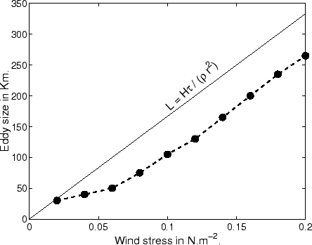 |
To characterize the size of the eddy as a function of wind stress, we
choose to measure the distance between the tip of the cape and the place where
the flow is the strongest towards the coast. The along shore eddy length given
by this method is proportional to the wind stress (figure
2.6) and the trend is in agreement with the characteristic
length scale found in section 6.2 (figure 2.5-a,
2.5-b, 2.5-c and 2.6).
There is though an approximately constant discrepancy ( km)
between the numerical results and the characteristic length scale, that reveals
that something is missing in deriving the analytical length scale.
Within the eddy, the flow is weak and the along shore velocities are positive
for
km)
between the numerical results and the characteristic length scale, that reveals
that something is missing in deriving the analytical length scale.
Within the eddy, the flow is weak and the along shore velocities are positive
for  km and
  km and negative around
  km. The constant
nature of this pattern might be related to the slope of the shelf or to the
size of the cape.
Ten more numerical experiments with wind stress fixed at were
conducted to explore the effects of the linear bottom friction coefficient.
This parameter varies from
km. The constant
nature of this pattern might be related to the slope of the shelf or to the
size of the cape.
Ten more numerical experiments with wind stress fixed at were
conducted to explore the effects of the linear bottom friction coefficient.
This parameter varies from
 m.s to
 m.s. For
low bottom friction values, the solution was not yet stationary at day 50, so
day 100 is analyzed.
m.s. For
low bottom friction values, the solution was not yet stationary at day 50, so
day 100 is analyzed.
Figure 2.7:
Barotropic velocities and sea surface elevation at day 100
forced by a constant wind stress (0.05 N.m), for different values of
the linear bottom coefficient r: a)
 m.s (maximum
velocity: 129 cm.s, averaged velocity: 49 cm.s), b)
m.s (maximum
velocity: 129 cm.s, averaged velocity: 49 cm.s), b)
 m.s (maximum velocity: 35 cm.s, averaged
velocity: 14 cm.s), c)
m.s (maximum velocity: 35 cm.s, averaged
velocity: 14 cm.s), c)
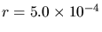 m.s (maximum
velocity: 19 cm.s, averaged velocity: 8 cm.s). The horizontal
coordinates are in kilometers and the greyscale range for the free surface
elevation is in centimeters. The interval between the isolines is 10 cm for
(a), 4 cm for (b), and 2 cm for (c).
m.s (maximum
velocity: 19 cm.s, averaged velocity: 8 cm.s). The horizontal
coordinates are in kilometers and the greyscale range for the free surface
elevation is in centimeters. The interval between the isolines is 10 cm for
(a), 4 cm for (b), and 2 cm for (c).
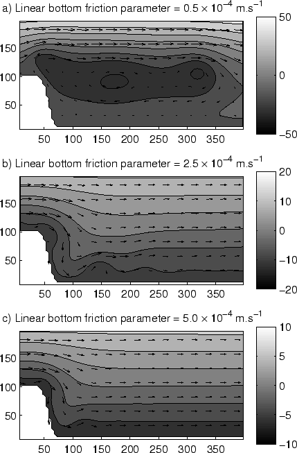 |
The mean velocities are again in the same order of magnitude
as predicted by the analytical calculations (figure 2.7). As
in the previous section, the different characteristic velocities and
characteristic parameters are derived. For increasing r, they follow the
range:
Again the Rossby and Ekman numbers are small and the viscous Reynolds number
is very large. But for this set of experiments, the frictional Reynolds number
which is the most important in the control of the detachment process, varies
through two orders of magnitude. Because this number is equivalent to the island
wake parameter of Wolanski et al. [1984], we can expect a
domination of bottom friction for low values and instabilities for large
values. For low bottom friction, the along shore size of the eddy does not match
the characteristic length scale and three small eddy cells keep on moving
inside a global structure(figure 2.7-a). The solution is not
yet steady at day 100 and different dynamical balances should exist. It appears
that in this experiment, we are in a eddy shedding regime.
Figure:
Along shore extension of the eddy at day 100 as a function of
the linear bottom friction parameter r. Comparison with the characteristic
length scale:
.
 |
For  m.s and corresponding
 , the eddy
size does scale with
, the eddy
size does scale with  (figure 2.8), but as in the
previous section this
size is not in agreement with the characteristic length scale.
This analysis confirms the key role of bottom friction in controlling the
detachment processes and the importance of parameterizing it carefully.
(figure 2.8), but as in the
previous section this
size is not in agreement with the characteristic length scale.
This analysis confirms the key role of bottom friction in controlling the
detachment processes and the importance of parameterizing it carefully.
3 Influence of the size of the cape
To explore the influence of the size of the cape on the detachment process, a
set of experiments has been conducted with a size of the cape ranging from 25
km to 150 km and a wind stress ranging from 0.025 N.m to 0.2 N.m.
The cross-shelf width of the periodical channel has been extended up to 300 km
in order to contain the biggest capes. The bathymetry has been computed in such
a way that the distance between the tip of the capes and the shelf break
remains identical between all the experiments. This implies that the width of
the shelf in the bay varies with the size of the cape (figure
2.9). The other parameters remain identical to the reference
experiment.
Figure 2.9:
Bottom topography implemented in the model for (a) a cape of 150 km
and (b) a cape of 25 km. The horizontal coordinates are in kilometers. The
depths scale is in meters.
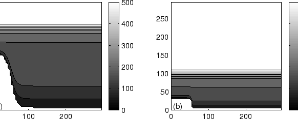 |
In every case, the solution is stationary after 50 days and remains in the
attached cyclonic eddy regime. The free surface elevation and the currents at
day 100 for a wind stress of 0.1 N.m reveal large differences depending
on the size of the cape (figure 2.10):
- In the bay, the drag induced by the presence of the cape produces an
averaged weaker current as the size of the cape increases. This averaged
velocity ranges from 32 cm.s for a cape of 25 km to 22 cm.s
for a cape of 50 km (for a wind stress of 0.1 N.m).
- The shelf break acting as an offshore barrier, mass conservation
implies a stronger current at the tip of the cape for a larger cape than for smaller
ones. The velocities at the tip of the cape range from 56 cm.s
for a cape of 25 km to 80 cm.s for a cape of 150 km (for a wind stress
of 0.1 N.m).
- These large differences in velocity, imply that a
scaling of the eddy length only dependent on the wind stress is no longer valid:
large variations in the size of the eddy depends on the size of the cape (see
figure 2.10 and figure 2.11).
Figure 2.10:
Barotropic velocities and sea surface elevation at day 100
forced by a constant wind stress (0.1 N.m), for different sizes of
the cape.
a) Cape of 25 km (maximum velocity: 56 cm.s, averaged
velocity: 32 cm.s).
b) Cape of 75 km (maximum velocity: 68 cm.s, averaged velocity:
29 cm.s).
c) Cape of 150 km (maximum velocity: 80 cm.s, averaged velocity:
22 cm.s).
The horizontal coordinates are in kilometers and the greyscale
range for the free surface elevation is in centimeters. The interval between
the isolines is 8 cm.
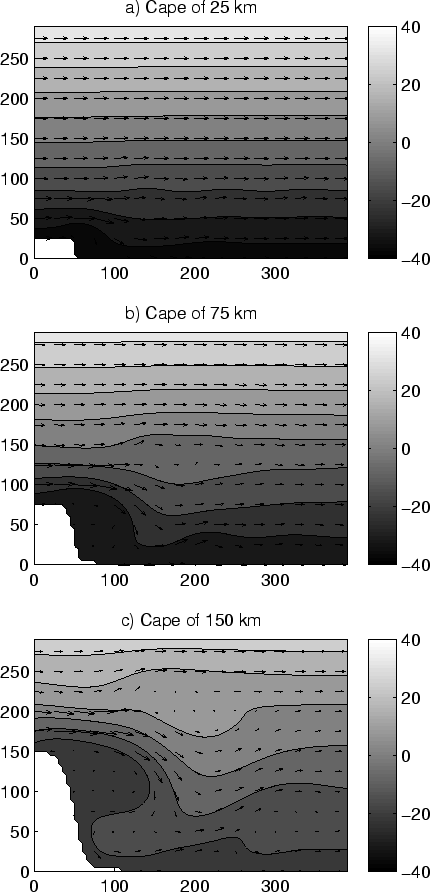 |
The difference between the size of the eddy and the frictional characteristic
length scale increases when the size of the cape decreases (figure
2.11). The balance advection / bottom friction is less valid for
small capes. This can be explained by the reduction of the importance of the
flat area in the lee of the cape for small capes (zero for a cape of 25 km, see
figure 2.9). Because the sloping areas are relatively more
important, the vortex stretching term gain importance relative to the bottom
friction term when the size of the cape decreases. For a cape of 25 km, the
size of the eddy as a function of the wind stress follows a totally different
trend than for the other experiments. For large capes ( 100 km), the
characteristic length scale gives a good approximation for the size of the
eddy as a function of the wind stress.
Figure 2.11:
Size of the attached cyclonic eddy as a function of the wind stress
and the size of the cape.
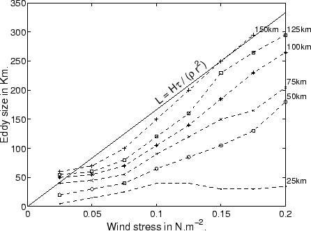 |
The size of the cape affects dramatically the recirculation
patterns in the bay. The length scale derived in section (2.5.2)
does not take the size of the cape into account. Hence, further investigations
will be necessary to improve the understanding of the circulation in the bay.
In section 1.4.4, it has been emphasized that a characteristic
pattern in St. Helena Bay is the development of an upwelling plume
from the tip of Cape Columbine. Numerous studies have been conducted to explain
the presence of this upwelling plume due to the cyclonic wind stress curl measured
in the lee of the cape [Jury, 1985a,Jury, 1985b,Jury, 1988,Kamstra, 1985,Taunton-Clark, 1985]. Although
cyclonic wind stress curl might be important in this area, and locally
enhances upwelling, none of these studies were able to model or
quantify the impact of wing stress curl on the upwelling structure. This has
been done, using a one and a half layer reduced-gravity model for the upwelling
of Point Arena on the US West Coast by Enriquez and Friehe [1995]. Although
their model produced an enhanced upwelling due to the presence of cyclonic wind
stress curl, it didn't generate a marked upwelling plume extending from the
cape.
In this section, I would like to propose the 'barotropic coastal flow
detachment' as another possible process for the generation of the Cape
Columbine upwelling plume. To illustrate this hypothesis, a 'barotropic'
tracer has been
introduced in the model to roughly simulate the sea surface temperature. It
follows an advection equation:
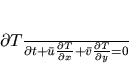 |
(22) |
To avoid the generation of numerical noise, biharmonic viscosity has been
added. At the model initialization, the value of the tracer is 20 everywhere,
except on a narrow band of 10 km at the tip of the Cape (x 30 km, y =110 km)
where it has a value of 10, accounting for the coastal upwelling. During all
the simulation, the tracer is nudged towards 10 in this band. Although the
offshore Ekman drift is not taken into account, this experiment is performed
to simulate the characteristic sea surface temperature pattern
observed in St Helena Bay.
Figure 2.12:
'SST' tracer after 30 days in a experiment forced by a wind stress of
0.05 N.m. The advection of low values of the tracer by the detached
flow simulate the Cape Columbine upwelling plume. The interval between the
isolines is 2.
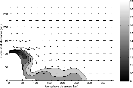 |
The tracer has been tested in a simulation forced by a constant wind stress of
0.05 N.m, the other parameters remaining as in the reference
experiment. After 30 days, even with this low wind forcing, a tongue of low
'SST' extends from the tip of the cape following the cyclonic eddy (figure
2.12). The shape of this tongue can be compared to a sea
surface portrayal of the Cape Columbine upwelling plume (figure
1.10). Thus, the horizontal advection of water upwelled South
of Cape Columbine around the attached cyclonic eddy can be an explanation of the
development of the Cape Columbine upwelling plume. Wind stress curl is not
necessary for the generation of this plume.
Another interesting feature is the patch of low tracer value at the coast at
120 km downstream from the cape (figure 2.12). This seems
to be related to wave like features visible in the currents downstream of the
main perturbation. Perhaps, there is here a possible explanation for the
presence of the Hondeklip Bay upwelling center.
8 Standing coastal trapped waves in the lee of Cape Columbine
The discrepancies between the characteristic length scale and the size of the
eddy shown on figure (2.11) suggest that a balance between
advection and bottom friction is not enough to describe the flow patterns in
the Bay. Other processes may also contribute actively. Two indications reveal
that the circulation observed in the lee of the cape might be related to
standing coastal trapped waves. Firstly, a wave-like pattern can be seen along
the coast, downstream of the cape (figure 2.2 for x 200 km).
Secondly, if we reverse the forcing and the topography orientation (i.e. for a
poleward eastern boundary current, figure 2.13), there is no
more detachment of the flow. This dissymetry is characteristic of a poleward
propagating process that can create a standing perturbation if it is advected
by a mean equatorward flow. Two candidates correspond to the 'poleward
propagation along a coastal eastern boundary' requirement: Kelvin waves and
coastal trapped waves.
Figure 2.13:
Barotropic velocities and free surface elevation at day 100 for a
'reversed' experiment where the wind stress of 0.05 N.m is poleward.
The topography orientation is also reversed. The maximum velocity is 38.5
cm.s and the averaged velocity is 14 cm.s.
The horizontal coordinates are in kilometers and the greyscale range for the
free surface elevation is in centimeters. The interval between the isolines is
2 cm.
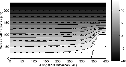 |
For the last three decades, coastal trapped waves have been studied
intensively. Buchwald and Adams [1968], derived the linear barotropic equation
of motion on a f plane for along shore propagating waves. The variation of
topography being of importance across the shelf, they kept the non-linear terms
in the vertically integrated equation of continuity. Because they were looking
for phenomena with spatial scales much smaller than the external radius of
deformation, the rigid lid approximation was made. In this case, the
cross-shelf structure of along shore propagating waves on an exponential
topography follows a linear second order differential equation. In the Northern
hemisphere, those free waves only propagate keeping the coast on their right
(on their left in the southern hemisphere). The generation of these waves by
atmospheric forcing has been analyzed by Gill and Schumann [1974] and they
found that resonance can occur with propagating wind perturbations. By keeping
the horizontal divergence, Huthnance [1975], derived 3 different kinds of
barotropic trapped waves over the continental shelf: the Kelvin waves that
propagate at the speed of long gravity waves, the edge waves with frequencies
higher than f, and the coastal trapped waves of sub inertial frequencies. It
happened that whereas edge waves may travel along the shelf in either
direction, Kelvin and coastal trapped waves progress along the shelf in a
cyclonic sense about the deep sea. There is a frequency at which the group
velocity of coastal trapped waves vanishes. At this frequency, the wave energy
cannot propagate along the shelf [Huthnance, 1975]. By including stratification,
Huthnance [1978] showed analytically and numerically that the coastal trapped
wave frequency increases with the measure of stratification. For weak
stratification (small Burger number), these waves take the form of barotropic
continental shelf waves, whereas for large stratification they take the form of
internal Kelvin waves. For large along shore wavenumbers they take the form of
bottom-trapped waves.
The presence of a mean along shore flow can alter considerably the free wave
properties by Doppler shifting and change in the background vorticity
[Brink, 1991,Huthnance, 1981]. Martell and Allen [1979] have studied the generation of
continental shelf waves by small along shore variations in bottom topography.
They used a perturbation method and found that shelf waves can be forced by the
interaction of a wind stress forced current with small topographic
disturbances. The advective effects of the unperturbed velocities are of
importance, and lee waves form when their phase velocity opposes the advective
velocities. The generation of lee waves is accompanied by a drag on the
topographic obstacle. The influence of the presence of a cape in scattering
coastal trapped waves has been explored analytically in the barotropic case
[Wilkin and Chapman, 1987] and numerically when stratification has been included
[Wilkin and Chapman, 1990]. In the barotropic case, reflection occurs when a wave
encounters a narrowing shelf. When the shelf widens, the energy is
transfered into higher modes and a shadow zone of very weak currents is
present in the vicinity of the cape. Its extent increases with the size of the
cape and decreases as the inverse of the wave frequency [Wilkin and Chapman, 1987]. When
stratification is added, scattering is found to be amplified and
intensification of the flow occurs within the scattering region [Wilkin and Chapman, 1990].
The influence of the advection by a mean current has not been taken into
account in these last studies.
Coastal trapped waves have been observed along the coast of South Africa from
tide gauges and current meters measurements. They propagate at a celerity
ranging from 4.2 m.s to 6.7 m.s. They induce variations in
sea level up to 50 cm and strong current reversals along the South Coast. The
Agulhas current damps dramatically wave propagation in the South-East
[Schumann and Brink, 1990]. Large scale stationary features of the Benguela front observed
from satellite imagery have been related to the existence of barotropic shelf
waves; but their standing nature has not been explained [Shannon, 1985].
The ingredients for standing lee shelf waves generation are present in the
barotropic numerical experiments conducted in this chapter. The wave guide is
formed by the shelf and the shelf edge slopes, the interactions between the
wind forced current and Cape Columbine can provide the forcing mechanism, and
the mean equatorward current allows the presence of a standing solution. Hence,
the recirculation process in the lee of Cape Columbine could be related to the
presence of lee shelf waves.
2 Wave lengths selected by a mean along shore current
The problem can be summarized has follow: what are the effects of the
interactions between a large cape like Cape Columbine and a mean wind forced
along shore current, on the circulation on the shelf in the lee of the cape ?
The interactions between a cape and a mean along shore current of
constant velocity  are approximately equivalent to the interactions
between a cape that moves in the opposite direction (with a velocity
are approximately equivalent to the interactions
between a cape that moves in the opposite direction (with a velocity  ) and
a fluid at rest. If
) and
a fluid at rest. If  are the Eulerian coordinates in the fix
referential and
are the Eulerian coordinates in the fix
referential and
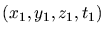 are the coordinates in the referential
attached to the moving cape, the temporal derivations have to be rewritten in
the moving frame:
are the coordinates in the referential
attached to the moving cape, the temporal derivations have to be rewritten in
the moving frame:
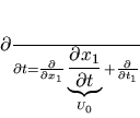 |
(23) |
For an observer moving with the cape, in the absence of wind stress, the
vertically averaged momentum equation (2.15) and the
continuity equation (2.4) take the form (removing the
subscripts for the coordinates):
With the variables
 made dimensionless by the characteristic values defined in
section (2.4)
made dimensionless by the characteristic values defined in
section (2.4)
 (
( is a characteristic time scale, days), equations
(2.24) leads to:
is a characteristic time scale, days), equations
(2.24) leads to:
where  and
and  are the Rossby and the vertical Ekman
numbers defined in section (2.4),
are the Rossby and the vertical Ekman
numbers defined in section (2.4),
 is
the horizontal Ekman number associated to the biharmonic operator, and
is
the horizontal Ekman number associated to the biharmonic operator, and
 is the external Rossby radius of deformation. In the
regime of parameters of the reference experiment (section 2.4),
is the external Rossby radius of deformation. In the
regime of parameters of the reference experiment (section 2.4),
 , , and
  are small compared to 1.
  400 km
is greater than the characteristic length scale
400 km
is greater than the characteristic length scale  (100 km) of our
problem, allowing the use of the rigid lid approximation. Although no
constraint is given on the value of in comparison to
(100 km) of our
problem, allowing the use of the rigid lid approximation. Although no
constraint is given on the value of in comparison to  , equations
(2.25) are linearized keeping the term of advection of momentum
by . Hence the dimensional remaining equations of motion are:
, equations
(2.25) are linearized keeping the term of advection of momentum
by . Hence the dimensional remaining equations of motion are:
Equations (2.26) show that we are looking for a
standing
process looking from the point of view of a moving cape. The resulting vorticity
equation takes the form:
 |
(27) |
where the vortex stretching balances the advection of vorticity due to
the displacement of the frame. Because bottom topography is defined in the fixed
referential, it does not make sense that variations of bottom topography move
from the cape point of view. Hence, H must not be variable in the along shore
direction. Equation (2.27) becomes:
 |
(28) |
The continuity equation in (2.26) is not divergent
for the transport and allows us to define a transport stream function of the form:
 |
(29) |
 |
(30) |
Introducing the transport stream function into the vorticity
equation (2.28) yields to:
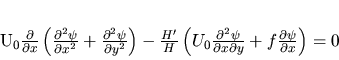 |
(31) |
The vorticity equation (2.31) can be linearized as
done by Wilkin and Chapman [1987] by using a bathymetry that follows an
exponential function:
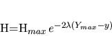 |
(32) |
Where  is the position of the offshore boundary. This gives:
|
(33) |
Equation (2.33) accepts solutions in the form of
standing shelf waves:
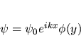 |
(34) |
Introducing the wave solution (2.34) into
(2.33) gives for  :
:
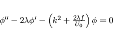 |
(35) |
As in section (2.2) an the analysis of Wilkin
and Chapman [1987], we will suppose that the offshore boundary is closed by a
wall at  . It has been demonstrated that the presence of a wall at
the shelf edge does not affect dramatically the shelf wave structure and
dispersion relation [Wilkin and Chapman, 1987]. For the sake of mass conservation,
. It has been demonstrated that the presence of a wall at
the shelf edge does not affect dramatically the shelf wave structure and
dispersion relation [Wilkin and Chapman, 1987]. For the sake of mass conservation,  must be constant along the walls in y=0 and . For , this is
only possible if
must be constant along the walls in y=0 and . For , this is
only possible if
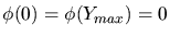 . This implies that the standing
shelf waves do not produce any net transport. The solution for equation
(2.35) that satisfies these boundary conditions is:
. This implies that the standing
shelf waves do not produce any net transport. The solution for equation
(2.35) that satisfies these boundary conditions is:
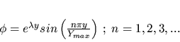 |
(36) |
Introducing the solution (2.36) into equation
(2.35) selects an along shore wavenumber for each mode in the form:
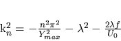 |
(37) |
The full solution of the vorticity equation (2.33) can
be write in the form of a sum of standing waves:
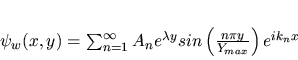 |
(38) |
In the Southern Hemisphere, the Coriolis parameter f is negative.
Thus, equation (2.37) implies that lee shelf waves can form only for
positive , accounting for an equatorward eastern boundary current. A
more general condition for the presence of a lee shelf wave of mode n is:
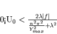 |
(39) |
If the relation (2.39) is not satisfied,  is imaginary
and the wave is evanescent. For
is imaginary
and the wave is evanescent. For
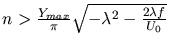 only evanescent
waves can be generated. Following Lighthill [1966], lee waves produced by a
moving perturbation have to propagate at a phase velocity equal to the speed of
the perturbation. Taking the propagating wave solution of Wilkin and Chapman
[1987], we obtain
only evanescent
waves can be generated. Following Lighthill [1966], lee waves produced by a
moving perturbation have to propagate at a phase velocity equal to the speed of
the perturbation. Taking the propagating wave solution of Wilkin and Chapman
[1987], we obtain
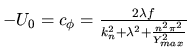 , which is identical to equation
(2.37). The condition (2.39) says that standing lee shelf wave
can only exist if is opposite to the shelf wave propagation and smaller
than the fastest shelf wave phase celerity.
Following the same approach of the section (2.5.2) , the wind
forced characteristic velocity defined by equation (2.9) can
give a reasonable value for in equation (2.37).
We obtain a standing shelf wave length
, which is identical to equation
(2.37). The condition (2.39) says that standing lee shelf wave
can only exist if is opposite to the shelf wave propagation and smaller
than the fastest shelf wave phase celerity.
Following the same approach of the section (2.5.2) , the wind
forced characteristic velocity defined by equation (2.9) can
give a reasonable value for in equation (2.37).
We obtain a standing shelf wave length  for each mode as a
function of the wind stress:
for each mode as a
function of the wind stress:
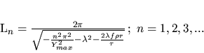 |
(40) |
To compare this result to the outputs from the previous
experiments, the topographic parameters have been chosen:
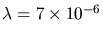 ,
,  km and
  m, so that the exponential
topography is relatively close to the bathymetry of the numerical model in St.
Helena Bay (2.2) (figure 2.14).
m, so that the exponential
topography is relatively close to the bathymetry of the numerical model in St.
Helena Bay (2.2) (figure 2.14).
Figure 2.14:
Comparison between the topography in the bay described in section
(2.2)(dotted line) and the exponential topography for
m and
(dashed line).
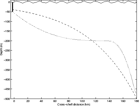 |
The wavelengths of the first two modes are of the same order of
magnitude as the size of the perturbations observed in the lee
of the cape (for a cape of 100 km)(figure 2.15). Thus the
detachment process is likely to be related to the presence of these standing
shelf waves. Nevertheless, these wavelengths increase when the
width of the shelf () decreases. This is in disagreement with the
pattern observed in section (2.6.3).
Figure 2.15:
Standing wave lengths for first 6 modes as a function of wind
stress for a bay of 180 km wide ( m and
). Comparison with the size of the eddy for a cape of 100 km.
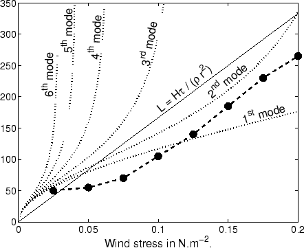 |
In this section, I would like to propose and illustrate a possible process for
standing waves excitation in the lee of a cape. To do so, the linear
vorticity equation (2.27) is supposed valid even in the close
vicinity of the cape. This linear problem implies that the moving cape does not
carry in its movement any water in its wake, and thus does not generate any net
transport. Because the cape moves in a channel bounded by a wall offshore, mass
conservation implies that, looking from the frame related to the cape, the
current in front of the tip of the cape is greater than the current ()
associated to the motion of the cape. The velocities at the tip of the cape are
supposed constant and equal to  . One can imagine that the flow is
redistributed inside a frictional boundary layer close to the cape. For
example, the lateral boundary layer thickness defined by Becker [1991],
dimensionalized by the size of the cape, is here around 5 kilometers. This is
one order of magnitude smaller than a characteristic wave length. If we keep
the topography defined in the previous section, global mass conservation for a
cape of cross-shelf extension
. One can imagine that the flow is
redistributed inside a frictional boundary layer close to the cape. For
example, the lateral boundary layer thickness defined by Becker [1991],
dimensionalized by the size of the cape, is here around 5 kilometers. This is
one order of magnitude smaller than a characteristic wave length. If we keep
the topography defined in the previous section, global mass conservation for a
cape of cross-shelf extension  implies:
 |
(41) |
Giving as a function of :
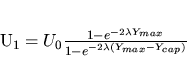 |
(42) |
The velocity () offshore of the cape and the presence of the
cape at x=0 imply that the along shore velocity, solution of the vorticity
equation (2.27), must have equal values at x=0 (in the frame moving
with the cape):
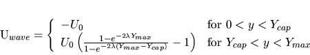 |
(43) |
This implies a wave solution in the same order of magnitude
of . Hence, the term
 has the same importance as the term
 in the addimentional momentum equation
(2.25). Solving the linear vorticity equation
(2.27), applying the boundary condition (2.43) for
x=0, is equivalent asking if a set of linear propagating waves can account for
the flow generated just at the back of a moving cape. The frictional boundary
layer is no longer necessary to explain the redistribution of the flow behind the
cape; this can be done by a set of linear standing waves. The boundary
condition at x=0 for the transport stream function accounting for the lee
shelf waves is:
in the addimentional momentum equation
(2.25). Solving the linear vorticity equation
(2.27), applying the boundary condition (2.43) for
x=0, is equivalent asking if a set of linear propagating waves can account for
the flow generated just at the back of a moving cape. The frictional boundary
layer is no longer necessary to explain the redistribution of the flow behind the
cape; this can be done by a set of linear standing waves. The boundary
condition at x=0 for the transport stream function accounting for the lee
shelf waves is:
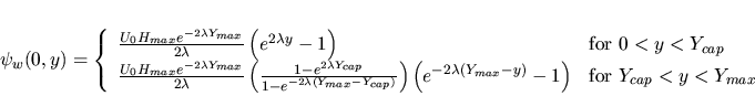 |
(44) |
One can note that  is continuous and that
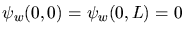 , in agreement with the properties of the standing
waves. For the following we will define
, in agreement with the properties of the standing
waves. For the following we will define
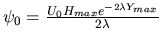 and
and
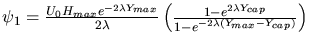 .
For x=0, pressure and transport should be both continuous. In this case,
although pressure can be obtained from the along shore momentum equation,
there is no information for the pressure for
.
For x=0, pressure and transport should be both continuous. In this case,
although pressure can be obtained from the along shore momentum equation,
there is no information for the pressure for  . This information could
be obtained by deriving also a wave solution upstream of the Cape (where
the mean current is ). To stay simple, we will keep only local
conservation of the transport for the matching conditions at x=0. This gives:
. This information could
be obtained by deriving also a wave solution upstream of the Cape (where
the mean current is ). To stay simple, we will keep only local
conservation of the transport for the matching conditions at x=0. This gives:
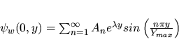 |
(45) |
Because
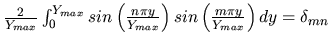 , we obtain:
 |
(46) |
Introducing the value of  :
:
 |
(47) |
With,
 |
(48) |
To confirm the validity of the assumptions made previously, a numerical
experiment using SCRUM has been conducted. The configuration is the same as the
reference experiment described in the section (2.4), except for the
bottom topography and the value of the wind forcing. In this experiment, the
bottom topography follows the equation (2.32) with
m and
(see figure 2.14). The
value of the constant wind stress is fixed at 0.05 N.m. The solution is
stationary after 50 days, thus a transport stream function can be extracted
from the model outputs. The transport stream function and the barotropic
velocities in the lee of the cape, for the model at day 100, are shown on
figure (2.17-a). Using this topography, no recirculation is
visible, the current follows the lee side of the cape to fill the bay.
Nevertheless, large standing waves remain in the lee of the cape. They exhibit
wave lengths ranging from roughly 50 km in the bay up to 100 km for the small
oscillations visible near the offshore boundary. The averaged value of the
along shore velocities is 0.1 m.s, which is 40 % less than the wind
forced velocities expected if there was no coastline variations (equation
2.9). This accounts for the drag induced by the cape on the
wind forced circulation. The wave pattern is rapidly damped with increasing x,
and oscillations are hardly visible after 3 wave lengths. The total transport
is about 3.5 Sv. The transport isocontour closest to the coast is moving
slightly offshore with increasing x, due to the presence of the downstream cape
associated to the periodic channel.
Figure 2.16:
Properties of the standing waves. a: Wavelengths in kilometers for the
20 first modes; the black dots accounts for the evanescent waves (in this
case, it is the e-folding length that is represented). b: Amplitude relative
to the first mode in percent of the 20 first modes; note that the seventh mode
amplitude is already less than 1% than the first mode amplitude. c: Total
difference in percent between the boundary condition and the wave solution in
x=0; there is less than 10% difference after 17 modes added.
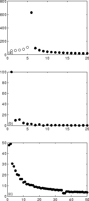 |
The mean along shore velocities of the numerical experiment (0.1
m.s) gives the value for for the calculation of the standing wave
solution. In this case, only the 5 first modes are non-evanescent. They
correspond to wave lengths ranging from 61 km to 110 km (figure
2.16-a). Evanescent waves adjust the solution to the
boundary condition close to the cape. Their amplitudes being small (figure
2.16-b), they do not strongly affect the solution in the bay.
The computation of the relative difference between the solution at x=0 and the
boundary condition (figure 2.16-c) shows that 17 modes are
sufficient to have a solution close to the boundary condition at x=0.
The graph (2.16-b) shows that most of the solution in the bay
is picked up by the first mode. The wave length of this mode is 61 km, which is
close to the value of the size of the eddy for this wind stress. The solution
given by summing the 20 first shelf waves modes and the mean along shore current
is represented on figure (2.17-b). The wave pattern close to
the cape and the waves length are consistent with the numerical result (figure
2.17-a), but no damping of the waves occurs in the bay. On the
contrary, variations happen to increase with increasing x in the first 300 km.
This difference is due to the absence of bottom friction when deriving the
wave solution. The effect of bottom friction can be roughly simulated by
introducing an exponential damping for each wave mode. A scaling of the effects
of bottom friction versus the advection by the mean current gives an e-folding
length  :
:
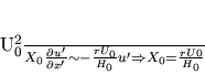 |
(49) |
Where is the mean value of the bottom topography and r is
the linear bottom friction parameter defined in section (2.2).
This gives an e-folding length of 50 km. The new solution is shown on figure
(2.17-c). It coincides relatively closely to the numerical
solution (figure 2.17-a). This result confirms the assumptions
made in deriving the standing waves equation and emphasizes the importance of
bottom friction. Another discrepancy is the difference between the numerical
and standing wave solutions for the incoming current at x=0. A remedy should
be to resolve the standing wave dynamics upstream of the cape and to add a
boundary condition on the free surface at x=0 as explained previously.
Figure 2.17:
Transport stream function and barotropic velocities in the lee of a
cape of 100 km width over an exponential bathymetry. a: Output at day 100 for
a numerical experiment forced by an along shore wind stress of 0.05
N.m. b: Standing waves solution for an along shore current  m.s. c: Same as b with the waves damped with an e-folding
along shore length of 50 km. In each portrayal, the interval between the
isolines is 0.5 Sv.
m.s. c: Same as b with the waves damped with an e-folding
along shore length of 50 km. In each portrayal, the interval between the
isolines is 0.5 Sv.
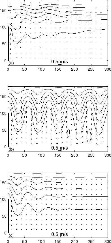 |
This analysis shows that a local mass conservation condition is sufficient to
generate standing waves forced by a mean current in the lee of a cape.
Although stratification is not taken into account, this may be an explanation
of the large scale stationary features observed in the upwelling front in the
lee of Cape Columbine [Shannon, 1985].
Whereas the presence of standing shelf waves and a balance advection/bottom
friction can explain the flow pattern in the lee of capes of an order of
magnitude of 100 km, this is not satisfactory in the case of small capes. For
small capes, perturbations develop in the bay close to shore, where the
bottom topography follows a law corresponding more to:
 |
(50) |
accounting for a flat shelf rising at the coast. Ball [1967], derived
the linear barotropic equations of motion over this topography for along shore
propagating waves with no offshore limit. He found solutions in the form of
edge waves. The same approach is applied in the case of standing waves.
Therefore, as in section (2.8.2), we look for solutions in the
standing wave form  , where
  is a function of y only. Introducing
this form for each variable in the linear equations of motion
(2.26), we obtain the system:
is a function of y only. Introducing
this form for each variable in the linear equations of motion
(2.26), we obtain the system:
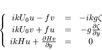 |
(51) |
Where all the variables are now only y-dependent. The solution of the
system (2.51) for (the linear vorticity equation) is:
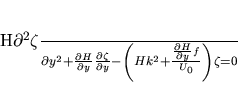 |
(52) |
with finite at the coast and zero at infinity. Introducing
the value of H and applying the variable transformation:
 |
(53) |
We obtain:
![\begin{displaymath}
s^2(1-s)\frac{\partial^2 \zeta}{\partial s^2}+
s(1-2s)\f...
...}{\lambda
U_0}-\frac{k^2}{\lambda^2}\right)s\right]\zeta = 0
\end{displaymath}](img299.png) |
(54) |
Following Ball [1967], this equation accepts solutions in the form:
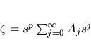 |
(55) |
where
 |
(56) |
and
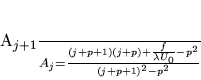 |
(57) |
In order to keep finite for
 , we must
have
, we must
have
 . The ratio (2.57) shows that the
series (2.55) is divergent unless it terminates. To terminates
the series, an integer n must exist such that:
. The ratio (2.57) shows that the
series (2.55) is divergent unless it terminates. To terminates
the series, an integer n must exist such that:
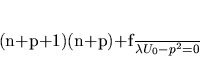 |
(58) |
Thus, selecting the wavelengths of the standing edge waves:
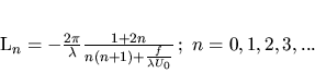 |
(59) |
Figure 2.18:
Standing edge wave lengths for the 4 first orders has a function of
the wind stress. Comparison with the size of the eddy for a cape of 25 km.
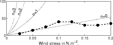 |
as been chosen equal
 to compare the result with
the size of the perturbation for a cape of 25 km. We can note on figure
(2.18) that the zero order edge wave length coincides with the
size of the eddy. This shows that smaller capes force this other kind of
waves. It explains the differences for the eddy size found between the
different
capes in figure (2.11).
To summarize, it has been demonstrated in this last section that although flat
bottom dynamics control the recirculation in the bay, topographic waves
are key phenomena in the barotropic detachment process on the shelf.
Because they occur only in presence of an equatorward current (at the eastern
boundary of an ocean), they can induce a dissymetry in the drag if the forcing
oscillates. This can produce a poleward net current in some places.
To illustrate the effects of the development of the eddy on the coastal and
offshore circulation, a tracer T has been introduced in the model. It follows
a time forced advective equation:
to compare the result with
the size of the perturbation for a cape of 25 km. We can note on figure
(2.18) that the zero order edge wave length coincides with the
size of the eddy. This shows that smaller capes force this other kind of
waves. It explains the differences for the eddy size found between the
different
capes in figure (2.11).
To summarize, it has been demonstrated in this last section that although flat
bottom dynamics control the recirculation in the bay, topographic waves
are key phenomena in the barotropic detachment process on the shelf.
Because they occur only in presence of an equatorward current (at the eastern
boundary of an ocean), they can induce a dissymetry in the drag if the forcing
oscillates. This can produce a poleward net current in some places.
To illustrate the effects of the development of the eddy on the coastal and
offshore circulation, a tracer T has been introduced in the model. It follows
a time forced advective equation:
 |
(60) |
The number 1 on the right of equation (2.60) is the
time forcing term. To be consistent with the numerical SCRUM model, the
equation (2.60) has been rewritten in the flux form and for the
sake of numerical stability, biharmonic viscosity has been included.
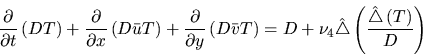 |
(61) |
has been kept as small as possible, and because in
all experiments  is of the order of
  , viscosity should
not perturb the solution. T is kept at zero at the upwind boundary. Away from
the boundary, T increments continuously. To test this, T has been introduced in
an experiment with a rectilinear coastline and a flat bottom. Using the former
analytical results, at day 50, when the solution is stationary (equation
2.9), the time since a water particle has left the upwind
boundary is only x-dependent:
, viscosity should
not perturb the solution. T is kept at zero at the upwind boundary. Away from
the boundary, T increments continuously. To test this, T has been introduced in
an experiment with a rectilinear coastline and a flat bottom. Using the former
analytical results, at day 50, when the solution is stationary (equation
2.9), the time since a water particle has left the upwind
boundary is only x-dependent:
 |
(62) |
The rectilinear coastline numerical experiment is in agreement with
this solution (figure not shown).
Figure 2.19:
Spatial distribution of the water age tracer at day 100 for
experiments similar to the reference experiment. The along shore wind stress is
fixed during each experiment at: (a) 0.05 N.m, (b) 0.1 N.m, (c)
0.15 N.m. The horizontal coordinates are in kilometers and the greyscale
range for the water age tracer is in days.The interval between the isolines is 5
days in each portrayal.
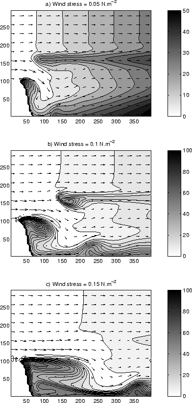 |
From the outputs at day 100 of the reference experiment, we can see that the
distribution of T over the model domain is strongly influenced by the
topography and the development of the eddy in the lee of the cape (figure
2.19-b). In the offshore area (y200 km), T increases almost
linearly towards
the right side of the domain (the downwind and equatorward directions), this
illustrates the advection of the water as it flows toward the equatorward side
of the model domain. In the coastal area, T reaches a maximum (90 days) in the
vicinity of the cape (x=40 km, y=100 km) and in the downstream near-shore area
(figure 2.19-b, T=60 days, x=80 km, y=90 km). It reaches a local
maximum
inside the shelf break meander where the velocities are weak (figure
2.19-b,
T=45 days, x=170 km, y=160 km). For a wind 50% stronger than the reference
experiment, whereas the area of strong T values has increased with the size of
the eddy, the maximal value of T does not vary significantly from the
reference experiment (figure 2.19-c). In this experiment, the
local
maximum on
the shelf edge has disappeared. For a wind 50% weaker, the eddy is small
(40 km) and its contribution does not affect dramatically the tracer
distribution (figure 2.19-a). Even so, there is a local
maximum
at the tip
of the cape (figure 2.19-a, T=40 days, x=45 km, y=95 km).
In order to investigate the effects of the intensity of the wind forcing on
the distribution of T, several successive runs of the model are performed
using values of wind stress increasing from 0.02 N.m to 0.2 N.m
by steps of 0.02 N.m (figure not shown). The spatial distribution of T
is extracted at day 50. For low wind forcing (ranging from 0.02 to 0.06
N.m) and weak flow detachment, there are small differences between the
coast and the offshore areas; T increases almost steadily over the entire
domain towards the right boundary. For moderate wind forcing ( ranging from 0.06
to 0.14 N.m), the eddy starts to develop downwind of the cape. In the
offshore area, the distribution of T is not affected by the eddy. In the
coastal domain, the development of the eddy induces an increase of the age of
the water retained in the eddy and on the coastal side of the eddy. T reaches a
maximum value of about 30 days in the near-shore domain. For strong wind forcing
( greater than 0.14 N.m), the size of the eddy growths as the wind but T
does not increase in the eddy
Figure 2.20:
Value of the water age tracer,  (a) and
  (b) at day
50 for values of wind stress forcing ranging from 0.02 N.m to 0.2
N.m by steps of 0.02 N.m.
(b) at day
50 for values of wind stress forcing ranging from 0.02 N.m to 0.2
N.m by steps of 0.02 N.m.
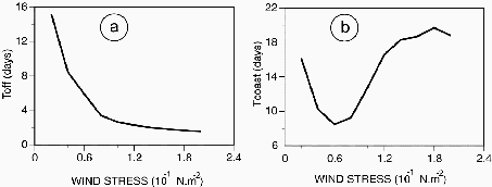 |
These results are summarized on figure 2.20. In order to allow
comparison
between the offshore and coastal regions, T is averaged over two areas: a
coastal/eddy area (T : x=25 to 150 km and y=0 to 110 km) and an
offshore area (T
: x=25 to 150 km and y=0 to 110 km) and an
offshore area (T : x=25 to 150 km and y=110 to 200 km). T and
T are calculated at day 50 for each of the successive runs performed
with wind stress ranging from 0.02 N.m to 0.2 N.m. In the
offshore domain, T decreases as an inverse function of the wind
stress: the stronger is the wind, the stronger is the advection towards the
right side of the model domain [e. g. equation (2.62)]. In the
coastal domain,
T decreases as the wind forcing increases from low to moderate (from
0.02 to 0.06 N.m). In that range of wind forcing, the cape has little
influence on the coastal circulation, the eddy size remains small compared to
the size of the cape. For stronger wind forcing, the effect of the eddy on the
coastal circulation is highly noticeable. For wind forcing ranging from 0.06 to
0.14 N.m, the size of the eddy expands and T increases
simultaneously with the wind. From 0.14 to 0.2 N.m, the size of the eddy
reaches or expands over the domain where T is calculated and
T reaches a plateau at a value of 18 days.
The variability of T and T over a wide range of wind forcing
illustrates the effects of the development of the eddy on the coastal and
offshore circulation. When the wind forcing is strong enough ( greater than
0.06 N.m), the eddy induces a pronounced recirculation in the coastal
domain, but the offshore area is unaffected. Looking back at
figure 2.2, one can see that while some water may enter the eddy
as a slow equatorward flow near-shore, most of the water has circulated around
the eddy and then entered from the bay side. The relative increase of T in the
coastal eddy domain, when compared to the value in the offshore area, is an
important consequence of the development of the eddy.
The presence of the eddy contributes to the formation of two distinct
patterns of circulation within the model domain: in the offshore area, the
circulation is predominantly along shore; in the coastal area, the circulation
is dominated by a cyclonic eddy and by the associated recirculation pattern.
The size of the eddy is positively related to the intensity of wind forcing.
The recirculation induced by the eddy tends to isolate the near-shore area from
the offshore domain. It limits the cross-shelf exchange of water and retains
water particles within the coastal domain, thus providing a mechanism for
retention. Retention in this coastal domain is then closely related to the
wind induced recirculation pattern. The next step in our analysis is to
evaluate the strength of retention as a function of the strength of the wind
forcing.
: x=25 to 150 km and y=110 to 200 km). T and
T are calculated at day 50 for each of the successive runs performed
with wind stress ranging from 0.02 N.m to 0.2 N.m. In the
offshore domain, T decreases as an inverse function of the wind
stress: the stronger is the wind, the stronger is the advection towards the
right side of the model domain [e. g. equation (2.62)]. In the
coastal domain,
T decreases as the wind forcing increases from low to moderate (from
0.02 to 0.06 N.m). In that range of wind forcing, the cape has little
influence on the coastal circulation, the eddy size remains small compared to
the size of the cape. For stronger wind forcing, the effect of the eddy on the
coastal circulation is highly noticeable. For wind forcing ranging from 0.06 to
0.14 N.m, the size of the eddy expands and T increases
simultaneously with the wind. From 0.14 to 0.2 N.m, the size of the eddy
reaches or expands over the domain where T is calculated and
T reaches a plateau at a value of 18 days.
The variability of T and T over a wide range of wind forcing
illustrates the effects of the development of the eddy on the coastal and
offshore circulation. When the wind forcing is strong enough ( greater than
0.06 N.m), the eddy induces a pronounced recirculation in the coastal
domain, but the offshore area is unaffected. Looking back at
figure 2.2, one can see that while some water may enter the eddy
as a slow equatorward flow near-shore, most of the water has circulated around
the eddy and then entered from the bay side. The relative increase of T in the
coastal eddy domain, when compared to the value in the offshore area, is an
important consequence of the development of the eddy.
The presence of the eddy contributes to the formation of two distinct
patterns of circulation within the model domain: in the offshore area, the
circulation is predominantly along shore; in the coastal area, the circulation
is dominated by a cyclonic eddy and by the associated recirculation pattern.
The size of the eddy is positively related to the intensity of wind forcing.
The recirculation induced by the eddy tends to isolate the near-shore area from
the offshore domain. It limits the cross-shelf exchange of water and retains
water particles within the coastal domain, thus providing a mechanism for
retention. Retention in this coastal domain is then closely related to the
wind induced recirculation pattern. The next step in our analysis is to
evaluate the strength of retention as a function of the strength of the wind
forcing.
Figure 2.21:
The relationship between the retention index  and wind stress,
ranging from 0.02 N.m to 0.2 N.m by steps of 0.02 N.m.
and wind stress,
ranging from 0.02 N.m to 0.2 N.m by steps of 0.02 N.m.
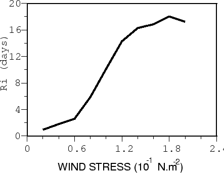 |
A true retention index would have been given by the residence time computed
from the advection fields provided by the model. However, the difference
between the age of the water in the coastal domain (T) and the
offshore
domain (T) can be used as a proxy to evaluate the intensity of the
retention. The variability of this index (further noted as ) gives an
indication on how the aging of the water differs between the two areas, a
positive (negative) value indicates water particles being older (younger) in
the coastal domain relative to the offshore area. From a biological point of
view, this offshore-inshore gradient can be used to evaluate the potential
advantage for larvae to be located in the coastal area. The variability of
as a function of wind stress is presented on figure
2.21.
increases
as the wind forcing increases, it reaches a maximum (18 days) value for a wind
stress of 1.8 N.m and then appears to level off or decrease. As
mentioned before, represents the difference between the coastal and the
offshore areas in the aging process of the water particles and should
not be used as an indicator of residence times within the bight.
This positive relationship between wind forcing and the retention index
suggests that, in an upwelling system, circulation patterns such as a standing
vortex may provide retention in the lee side of a cape. Further, stronger
upwelling favorable winds can enhance retention within the near-shore area
despite the intensification of the offshore flow related to the upwelling. Such
structures, providing a positive coupling between upwelling and retention, have
been documented in several upwelling systems [Graham and Largier, 1997,Roy, 1998].
In the Benguela upwelling system, most of the spawning occurs in late spring
and summer, during the peak season of the upwelling. Fish eggs and larvae are
transported from the spawning ground to the West Coast upwelling by a coastal
jet. With the classical wind-driven coastal upwelling circulation structure of
offshore transport of surface water, larvae will tend to be transported in the
offshore domain and be lost. However, our modeling experiment shows that the
Cape Columbine plume and the associated coastal recirculation in St Helena Bay
provide a retention mechanism allowing the larvae to be retained within the
productive coastal domain and thereby to avoid dispersion in the offshore
area.
We used an idealized numerical model to understand the interactions
between the wind-induced circulation on the shelf and topographical features
such as Cape Columbine and St. Helena Bay. The setting of the model is based
on the assumption that the circulation on the shelf follows barotropic
dynamics. Hence, the barotropic equations of motion have been solved in a
periodic channel and over an analytical bathymetry. They have been constrained
by a constant upwelling favorable wind stress and a linear bottom friction.
Despite these simplifications, it appears that the model is able to produce a
cyclonic eddy in St. Helena Bay that corresponds to the observed circulation
pattern [Holden, 1985,Shannon, 1985,Boyd and Oberholster, 1994]. The shape and size of this eddy
are in relative agreement with the results of Oey [1996] and Boyer
and Tao [1987a]. The eddy creates a dynamical barrier, limiting
the exchanges between the near-shore area and the shelf edge domain.
Diagnostic analysis shows that the recirculation process is controlled by a
balance between the Coriolis acceleration and the pressure gradient. The
velocities offshore are linked to a balance between wind stress and bottom
friction and the external part of the eddy follows cyclo-geostrophic dynamics.
When the numerical solution reaches a stationary state, a vorticity analysis
reveals that a balance between the curl of advection and the curl of bottom
friction controls the eddy dynamics. This balance gives a characteristic eddy
length scale proportional to the wind stress and inversely proportional to the
square of the linear bottom friction parameter. Several numerical experiments
using a wide range of wind stress and bottom friction values, indicate that the
along shore extension of the eddy follows the trends of this length scale when
the dynamics are in the attached-cyclonic-eddy regime. The influence of the
size of the cape has been tested, showing different regimes of perturbations.
Different kinds of standing coastal trapped waves, in equilibrium with a mean
along shore current have been proposed to explain the resulting flow patterns in
the bay. An analytical solution has been derived to explain the standing shelf
wave excitation by a mean along shore current past a cape.
A barotropic tracer representing the sea surface temperature has been
introduced into the model to illustrate the impact of an attached barotropic
cyclonic eddy on the generation of upwelling plumes
A tracer showing the age of the water is introduced to evaluate the
intensity of recirculation generated by the eddy in the coastal domain. This
tracer is used as a proxy for retention and to explore the relation between the
intensity of retention and wind forcing. In accordance with previous
observations, the model simulation indicates that the topography induces
retention in the lee side of the cape. In regions where fish spawning occurs
during the upwelling season, fish have successfully used such structures to
reproduce [Roy et al., 1989,Bakun, 1996,Bakun, 1998]. In the Benguela upwelling system, St Helena
Bay is recognized as the main nursery ground off the West coast where juvenile
fish are concentrated [Hutchings, 1992], suggesting that this retention mechanism
may be critical to recruitment success.
This idealized work provides a conceptualized portrayal of some typical
processes that we can encounter in St. Helena Bay.
3 A regional model of the South African West coast
Setting up a high resolution numerical model of the ocean circulation in the
surroundings of the South and West coasts of southern Africa was the direction
chosen by the VIBES project to explore the physical processes affecting fish, eggs,
larvae and juveniles during the recruitment cycle. This chapter provides a
description of the main characteristics of the numerical tools that were set up. A
detailed analysis of the numerical model output is provided and is aimed at
evaluating the validity of the modeling experiments. An illustration of the
potential use of such numerical tools in fisheries oceanography is provided by a set of
experiments designed to investigate the effect of transport on the fish spawning
products using a passive tracer.
Afin d'explorer les processus physiques affectant poissons,  ufs, larves et
juvéniles durant le cycle de reproduction, la direction choisit par le projet
VIBES consistait en la mise au point d'un modèle numérique à haute résolution
de la circulation océanique autour des côtes Sud et Ouest de l'Afrique australe.
Ce chapître apporte la description des caractéristiques principales des outils
numériques développés. Une analyse détaillée des sorties du modèle
numérique est conduite et est employée afin d'évaluer la validité des solutions.
Une illustration de l'utilisation potentielle de ces outils numériques en
Océanographie des pêches est fournie par une suite d'expériences utilisant un traceur passif,
développées pour étudier les effets du transport sur les produits de la ponte des poissons.
Few attempts have been undertaken to model the shelf and slope dynamics around the
South and West coast of South Africa. Van Foreest and Brundrit [1982] developed a
two-mode linear numerical model using a Galerkin procedure for the vertical and
applied it to the South Benguela. The surface forcing was idealized (constant
northward wind stress), and the time of integration was short (3 days).
Nevertheless, the solution was showing the topographic steering of the baroclinic
jet of Cape Peninsula. More recently, the Princeton Ocean Model (POM), a sigma
coordinate model, has been applied to simulate the circulation around the Southern
Africa from about 46 S to 12 S and 4 E to 30 E [Skogen, 1998]. 18
bottom following
ufs, larves et
juvéniles durant le cycle de reproduction, la direction choisit par le projet
VIBES consistait en la mise au point d'un modèle numérique à haute résolution
de la circulation océanique autour des côtes Sud et Ouest de l'Afrique australe.
Ce chapître apporte la description des caractéristiques principales des outils
numériques développés. Une analyse détaillée des sorties du modèle
numérique est conduite et est employée afin d'évaluer la validité des solutions.
Une illustration de l'utilisation potentielle de ces outils numériques en
Océanographie des pêches est fournie par une suite d'expériences utilisant un traceur passif,
développées pour étudier les effets du transport sur les produits de la ponte des poissons.
Few attempts have been undertaken to model the shelf and slope dynamics around the
South and West coast of South Africa. Van Foreest and Brundrit [1982] developed a
two-mode linear numerical model using a Galerkin procedure for the vertical and
applied it to the South Benguela. The surface forcing was idealized (constant
northward wind stress), and the time of integration was short (3 days).
Nevertheless, the solution was showing the topographic steering of the baroclinic
jet of Cape Peninsula. More recently, the Princeton Ocean Model (POM), a sigma
coordinate model, has been applied to simulate the circulation around the Southern
Africa from about 46 S to 12 S and 4 E to 30 E [Skogen, 1998]. 18
bottom following  -layers are used in the vertical, and the horizontal
resolution is 20 km. We can note that a condition of zero barotropic velocities is
given for the initial and boundary conditions. The simulations are forced using
data of a specific year. The results showed most of the characteristic features of
the circulation of the Benguela, but the resolution was too coarse to resolve the
mesoscale characteristics patterns that develops on the shelf in the West Coast
area. Several basin-scale models had the Benguela included in their simulation
domains [Barnier et al., 1998,Biastoch and Krauß, 1999,Marchesiello, 1995,de Miranda, 1996]. But their resolutions were also too
coarse (1/3 of a degree for the bests) to provide a satisfactory circulation pattern
for the transport of eggs and larvae around the South and West coasts of South Africa .
The first developed oceanic primitive equation models were using for the vertical,
the geopotential coordinate z. In this case the bottom topography is represented by
steps in the grid. This was not satisfactory for the simulation of bottom flows
along the topography, of particular importance in coastal dynamics. Thus,
traditionally in coastal modeling, it has been preferred to use models in which the
vertical coordinate follows the topography.
For this study, we use ROMS (the Regional Ocean Modeling Systems), a community code
developed by the modeling groups at Rutgers University (USA) and at University of
California Los Angeles (USA). It belongs to a hierarchy of terrain-following models
originated with the semi-spectral primitive equation model (SPEM, [Haidvogel et al., 1991]),
which solves the hydrostatic primitive equations with a rigid lid at the sea
surface, coupled with advection/diffusion equations for potential temperature and
salinity and the nonlinear UNESCO equation of state. SCRUM (S-coordinate Rutgers
University Model), a free sea surface version of SPEM has been developed by Song and
Haidvogel [1994]. It improves upon SPEM by allowing for a generalized nonlinear
terrain-following coordinate, which provides enhanced resolution at either the sea
surface or sea floor. This feature might be of importance for the biology, since
biological activity occurs mostly in the surface oceanic layers. ROMS represents an
evolution of SCRUM, including several substantial developments required to
efficiently and robustly calculate the coastal circulations at high spatial
resolution, such as subgrid scale parameterization, high order schemes, and high
performance computing on SMP-class computer architecture (like the SGI Origin 2000
of the University of Cape Town).
The equations of motion in Cartesian coordinates, following the Boussinesq and
hydrostatic approximations, take the form:
-layers are used in the vertical, and the horizontal
resolution is 20 km. We can note that a condition of zero barotropic velocities is
given for the initial and boundary conditions. The simulations are forced using
data of a specific year. The results showed most of the characteristic features of
the circulation of the Benguela, but the resolution was too coarse to resolve the
mesoscale characteristics patterns that develops on the shelf in the West Coast
area. Several basin-scale models had the Benguela included in their simulation
domains [Barnier et al., 1998,Biastoch and Krauß, 1999,Marchesiello, 1995,de Miranda, 1996]. But their resolutions were also too
coarse (1/3 of a degree for the bests) to provide a satisfactory circulation pattern
for the transport of eggs and larvae around the South and West coasts of South Africa .
The first developed oceanic primitive equation models were using for the vertical,
the geopotential coordinate z. In this case the bottom topography is represented by
steps in the grid. This was not satisfactory for the simulation of bottom flows
along the topography, of particular importance in coastal dynamics. Thus,
traditionally in coastal modeling, it has been preferred to use models in which the
vertical coordinate follows the topography.
For this study, we use ROMS (the Regional Ocean Modeling Systems), a community code
developed by the modeling groups at Rutgers University (USA) and at University of
California Los Angeles (USA). It belongs to a hierarchy of terrain-following models
originated with the semi-spectral primitive equation model (SPEM, [Haidvogel et al., 1991]),
which solves the hydrostatic primitive equations with a rigid lid at the sea
surface, coupled with advection/diffusion equations for potential temperature and
salinity and the nonlinear UNESCO equation of state. SCRUM (S-coordinate Rutgers
University Model), a free sea surface version of SPEM has been developed by Song and
Haidvogel [1994]. It improves upon SPEM by allowing for a generalized nonlinear
terrain-following coordinate, which provides enhanced resolution at either the sea
surface or sea floor. This feature might be of importance for the biology, since
biological activity occurs mostly in the surface oceanic layers. ROMS represents an
evolution of SCRUM, including several substantial developments required to
efficiently and robustly calculate the coastal circulations at high spatial
resolution, such as subgrid scale parameterization, high order schemes, and high
performance computing on SMP-class computer architecture (like the SGI Origin 2000
of the University of Cape Town).
The equations of motion in Cartesian coordinates, following the Boussinesq and
hydrostatic approximations, take the form:
 |
 |
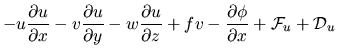 |
(63) |
 |
|
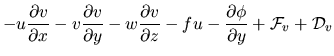 |
(64) |
 |
|
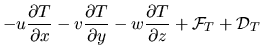 |
(65) |
 |
|
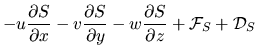 |
(66) |
 |
|
 |
(67) |
 |
|
 |
(68) |
 |
|
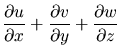 |
(69) |
With the vertical boundary conditions prescribed as follows:
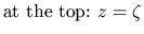 |
 |
 |
(70) |
| |
 |
 |
(71) |
| |
 |
 |
(72) |
| |
 |
 |
(73) |
| |
 |
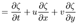 |
(74) |
 |
|
 |
(75) |
| |
|
 |
(76) |
| |
|
 |
(77) |
| |
|
|
(78) |
| |
|
 |
(79) |
Where,
- x, y, z are the coordinates in the Cartesian frame (z being
the vertical, increasing towards the top)
- u, v, w are components of the
velocity vectors in this frame
- f is the Coriolis parameter
- is the
dynamic pressure
 ,
,  ,
,  ,
,  are
the forcing terms
are
the forcing terms
 ,
,  ,
,  ,
,  are
the dissipation terms
are
the dissipation terms
- T is the potential temperature of the Ocean
- S is
the salinity of the Ocean
- P is the total pressure
 is the
total in-situ density
is the
total in-situ density
- g is the acceleration of gravity
- is the
free surface elevation
 ,
,  ,
,  are the vertical
turbulent mixing coefficients, defined by a vertical turbulent closure scheme
are the vertical
turbulent mixing coefficients, defined by a vertical turbulent closure scheme
 ,
,  are the surface wind stress components
 is the surface heat flux
 is the evaporation minus the precipitation
 ,
,  are the bottom stress components, the bottom
stress is parameterized in a sum of linear and quadratic terms:
are the bottom stress components, the bottom
stress is parameterized in a sum of linear and quadratic terms:
 |
(80) |
 |
(81) |
- H is
the resting thickness of the water column
Equations (3.1) and (3.2) express the momentum
balance in the x and y directions. Equations (3.3) and (3.4)
express the time evolution of Temperature and Salinity. Equation (3.5)
gives the non-linear equation of state. Under the hydrostatic approximation, the
momentum balance in the vertical direction limits itself to a balance between the
pressure gradient and the buoyancy forces (3.6). In the Boussinesq
approximation, density variations are neglected in the momentum equations except in
their contribution to the buoyancy forces in the vertical momentum equation
(3.6). Equation (3.7) expresses the continuity
equation for an incompressible fluid.
With an active sea surface, a generalized
topography-fitting coordinate takes the form:
 |
 |
|
(82) |
As an
extension to standard terrain-following transformations, a nonlinear stretching of
the vertical coordinate is applied that depends on local water depth [Song and Haidvogel, 1994].
It can be used to generate a more uniform vertical resolution near the surface (or
the bottom) and consequently a better representation of the mixed layer and the
thermocline. The transformation used in SCRUM and ROMS is:
 |
(83) |
where  is a constant to be chosen as a typical
surface mixed layer depth, and
is a constant to be chosen as a typical
surface mixed layer depth, and
![\begin{displaymath}C(s)=(1-\theta_b)\frac{\sinh(\theta
s)}{\sinh(\theta)}+ \the...
...ft[\theta(s+
1/2)\right]-\tanh(\theta/2)} {2 \tanh(\theta/2)} \end{displaymath}](img374.png) |
(84) |
For large  ,
the coordinate lines are more tightly confined to the surface; additionally, if
,
the coordinate lines are more tightly confined to the surface; additionally, if
 approaches 1, resolution at the bottom boundary is enhanced. These
possibilities might be of great importance for the coupling with the biological
components. The vertical velocity in the s coordinate is defined as:
approaches 1, resolution at the bottom boundary is enhanced. These
possibilities might be of great importance for the coupling with the biological
components. The vertical velocity in the s coordinate is defined as:
![\begin{displaymath}
\Omega = \frac{\partial s}{\partial z}\left[ w- (1+s) \frac...
...t)_s - v \left(\frac{\partial
z}{\partial y}\right)_s \right] \end{displaymath}](img377.png) |
(85) |
In the transformed coordinate system,
the kinematic boundary conditions (3.12) and (3.17), at the
surface  and at the bottom
  simplify to:
 |
(86) |
Figure 3.1:
Curvilinear coordinates.
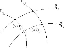 |
In the horizontal, like SPEM and SCRUM, ROMS is written in horizontal curvilinear
coordinates. This system can conform to irregular lateral boundaries or allows the
placing of more computational resolution in regions of interest. These new coordinates
are introduced by a transformation in the horizontal coordinate from (x,y) to
 , where the relationship of horizontal arc length to the differential
distance is given by:
, where the relationship of horizontal arc length to the differential
distance is given by:
Here,  and
and  are the scale factors which
relate the differential distances
are the scale factors which
relate the differential distances
 to the physical arc
lengths
to the physical arc
lengths
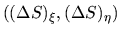 (figure 3.1).
Coastal boundaries can also be specified as a finite-discretized grid via land/sea
masking.
In the horizontal direction , except where noted below, a centered
second-order finite difference approximation is adopted on an Arakawa "C" grid
(figure 3.2), which is well suited for problems with horizontal
resolution that is fine compared to the first radius of deformation [Hedström, 1997].
(figure 3.1).
Coastal boundaries can also be specified as a finite-discretized grid via land/sea
masking.
In the horizontal direction , except where noted below, a centered
second-order finite difference approximation is adopted on an Arakawa "C" grid
(figure 3.2), which is well suited for problems with horizontal
resolution that is fine compared to the first radius of deformation [Hedström, 1997].
Figure 3.2:
Position of the variables on the Arakawa horizontal C-grid.
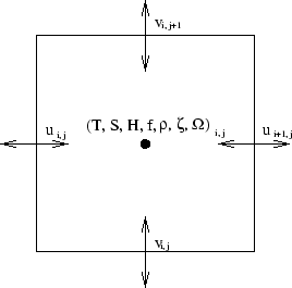 |
The vertical also uses a second-order finite-difference approximation. Just as we
use a staggered grid in the horizontal, the grid is staggered also in the vertical
(figures 3.3 and 3.4). These choices are traditional for
second-order, finite differences models, and provide for conservation of the first
and second moments of momentum and tracers [Haidvogel et al., 2000].
Figure 3.3:
Position
of variables on the staggered vertical grid.
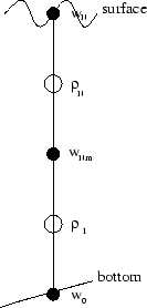 |
Figure 3.4:
Placement of variables on a ROMS cross section.
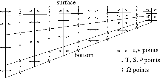 |
For computational economy, the hydrostatic primitive equations for momentum are
solved using a split-explicit time-stepping scheme which requires a special
treatment and coupling between barotropic (fast) and baroclinic (slow) modes. A
finite number of barotropic time steps, within each baroclinic step, are carried out
to evolve the free-surface and vertically integrated momentum equations. In order
to avoid the errors associated with the aliasing of frequencies resolved by the
barotropic steps but unresolved by the baroclinic step, the barotropic fields are
time averaged before they replace those values obtained with a longer baroclinic
step. A cosine-shape time filter, centered at the new time level, is used for the
averaging of the barotropic fields. In addition, the separated time-stepping is
constrained to maintain exactly both volume conservation and constancy preservation
properties which are needed for the tracer equations. Currently, all 2D and 3D
equations are time discretized using a third-order accurate predictor (Leap-Frog)
and corrector (Adams-Molton) time-stepping algorithm which is very robust and
stable. The enhanced stability of the scheme allows larger time steps than in more
traditional numerical scheme, by a factor of four, which more than offsets the
increased cost of the predictor-corrector algorithm.
4 The pressure gradient scheme
The major advantage of sigma coordinate models is the transformation of the surface
and sea bottom to coordinate surfaces. Unfortunately, this is also the source of
their major disadvantage: the well known pressure gradient error. In linear
coordinate, the x-component of the pressure gradient force is determined by the sum
of 2 terms:
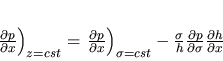 |
(89) |
The first term of the right involves the variation of pressure along a constant
-surface and the second is the hydrostatic correction. Near steep
topography, these 2 terms are large, comparable in magnitude and tend to cancel each
other. A small error in computing either term can result to a relatively large error
in the resulting horizontal pressure gradient [Song, 1998]. Another source of
error,
the hydrostatic inconsistency [Haney, 1991], can occur when using second order
central differences in the discretization of equation (3.27). It
can be demonstrated that the second order discretization of equation
(3.27) is equivalent to interpolating pressure between the
contiguous sigma layers to obtain the horizontal pressure gradient [Kliem and Pietrzak, 1999].
Hydrostatic inconsistency arises if the slope and horizontal resolution are such
that extrapolation is performed instead of interpolation. Kliem and Pietrzak [1999]
and Song [1998] proposed different ways to reduce errors:
- Reducing the truncation error in the derivation of equation
(3.27) by subtracting an horizontally homogeneous averaged density
 to the density field. This trick has an efficiency only for small
domains, where the horizontal variations in density are limited.
to the density field. This trick has an efficiency only for small
domains, where the horizontal variations in density are limited.
- Interpolating density back to z levels before computing the pressure gradient.
Problems can arise with the lowest and highest levels that could require
extrapolations over steep topography.
- Using higher-order numerical schemes.
- Retaining integral properties. The best pressure gradient formulation should
minimize truncation errors while retaining integral properties such as mass, energy
and vorticity.
The scheme implemented in ROMS is the weighted Jacobian formulation proposed by Song
[1998]. This formulation has been designed to minimize truncation errors and to
retain integral properties. If  is the generalized topographic following
coordinate system, the horizontal pressure gradient can be rewrite in a Jacobian
form:
is the generalized topographic following
coordinate system, the horizontal pressure gradient can be rewrite in a Jacobian
form:
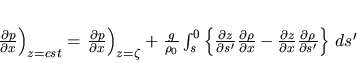 |
(90) |
Hence, vertical variations in the horizontal pressure gradient are given by an
integral of the Jacobian:
 |
(91) |
Song [1998] defined the standard Jacobian formulation as the second order central
difference discretization of equation (3.29). He proposed another scheme,
the weighted Jacobian, centered in z space rather than in s space, as for the
standard Jacobian. In an idealized case, Song [1998] shows that whereas the standard
Jacobian outperforms the weighted Jacobian when the hydrostatic consistency
condition is satisfied, the weighted Jacobian gives superior results if the
condition is violated (which is often the case in realistic configurations). The
conservation of momentum and energy and the accurate representation of the bottom
pressure torque
has been validated [Song and Wright, 1998]. The conservation of these properties can constrain
model errors.
A classic approach in Ocean modeling for the treatment of advection is the use
of second order central difference schemes. In conjunction, Laplacian, higher-order
diffusion operators or low-pass spatial filters are employed to smooth the numerical
noise induced by dispersive computational errors or turbulent cascades. The
advection operator for the momentum and tracer variables in ROMS has been redesigned
to reduce dispersive errors. It consists of an upstream-biased third order scheme.
Using this scheme, explicit smoothing of the fields is no longer mandatory, enhancing
the effective resolution of the solution for a given grid [Shchepetkin and McWilliams, 1998].
The parameterization of the unresolved physical vertical mixing processes in ROMS is
done via a non-local, K-profile planetary (KPP) boundary layer scheme [Large et al., 1994].
Two distinct parameterizations are conducted: one for the ocean interior and one for
the oceanic surface boundary layer. The boundary layer depth (h) depends on the
surface forcing, the buoyancy and the velocity profile and is determined by equating
a bulk Richardson number relative to the surface to a critical value. Below the
boundary layer, the vertical mixing is regarded as the superposition of 3 processes:
vertical shear, internal wave breaking, and double diffusion. In the surface layer,
the diffusivity is formulated to agree with a similarity theory of turbulence. At the
base of the surface layer, both diffusivity and its gradient have to match the
interior values. The KPP model has been shown to simulate accurately processes such
as convective boundary layer deepening, diurnal cycling, and storm forcing.
3 Configuration
1 The grids
Several arguments constrain the choices for the computational domain:
- the domain must be large enough so that the most important
dynamic features for the transport of eggs and larvae have enough space to develop.
This includes the upwelling filaments that extend several hundred of km offshore,
the Agulhas retroflection, etc...
- the domain must be small enough so that we
can keep a high resolution at a reasonable computational cost.
- the open
boundaries should cross the current at right angles. They should be placed where
there is a minimum in current velocities and in variability, they should also be
placed where the topographic gradient perpendicular to the boundary is as small as
possible to avoid along-boundary currents [Penduff, 1998].
Figure 3.5:
The
pie shaped grid for the low resolution experiment. The dark line represent the
coastline and the 500 m isobath is an indicator of the position of the shelf break.
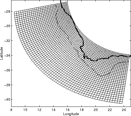 |
To satisfies these criteria, the grid has been
built following the arc of a circle. It follows roughly the South-west corner of
Africa and the resolution is identical in the  and
and  directions. This
way, the number of masked points, that are a dead weight in computing the
solution, has been reduced. To facilitate the connections to the open Ocean, the
Northern and Eastern open boundaries cut the shelf in its narrowest parts at about
respectively
directions. This
way, the number of masked points, that are a dead weight in computing the
solution, has been reduced. To facilitate the connections to the open Ocean, the
Northern and Eastern open boundaries cut the shelf in its narrowest parts at about
respectively  S and
S and  E. Hence, the model domain includes all the
South and South-West coasts of South Africa from Lüderitz to Cape St. Francis
(figure 3.5). The Eastern boundary is not at a place where the
currents are weak, since it cuts the strong Agulhas Current. We rely on a specific
open boundary scheme to handle this feature properly. The offshore boundary is placed
beynd
the shelf break, on the ocean plane, roughly 300 kilometers away from the tip of the
Agulhas Bank. This way, the domain is 1300 km long in its inner radius (at the
coast), 2240 km long offshore, and 740 km wide. Two kinds of grid have been realized:
E. Hence, the model domain includes all the
South and South-West coasts of South Africa from Lüderitz to Cape St. Francis
(figure 3.5). The Eastern boundary is not at a place where the
currents are weak, since it cuts the strong Agulhas Current. We rely on a specific
open boundary scheme to handle this feature properly. The offshore boundary is placed
beynd
the shelf break, on the ocean plane, roughly 300 kilometers away from the tip of the
Agulhas Bank. This way, the domain is 1300 km long in its inner radius (at the
coast), 2240 km long offshore, and 740 km wide. Two kinds of grid have been realized:
- a low resolution one where the resolution is linearly ranging
from 18 km at the coast to 31 km offshore.
- a high resolution one where the
resolution is linearly ranging from 9 km at the coast to 16 km offshore.
Note that the grid is isotropic and thus doesn't produce a dissymetry in the
dissipation of the turbulence. The resolution is higher at the coast where we need
a more accurate solution. The first baroclinic Rossby radius of deformation is
everywhere resolved in the high resolution experiment.
Although the pressure gradient scheme should allow the use of a steeper slope, some
degree of topographic smoothing may be necessary to ensure stable and accurate
simulations using realistic bathymetry. A useful parameter is found to be:
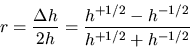 |
(92) |
Empirical studies
have shown that robust results are obtained if r does not significantly exceed a
value of 0.2 [Haidvogel et al., 2000]. To filter the topography only where it is needed, we
used a Shapiro filter weighted by the values of r: if r is smaller than a target
value (here, 0.15), the weight is 0; if r is bigger, the weight is 1. The filter
has been passed on the topography until  for the low resolution experiments
and until
for the low resolution experiments
and until  for the high resolution experiments. The low resolution
experiment has a bigger value because it was not possible to filter further the
topography at this resolution without removing all the shelf on the West Coast (see
for example figure 3.8).
for the high resolution experiments. The low resolution
experiment has a bigger value because it was not possible to filter further the
topography at this resolution without removing all the shelf on the West Coast (see
for example figure 3.8).
Figure 3.6:
Raw ocean
topography (greyscale range in meters) from the ETOPO2 dataset.
 |
Figure 3.7:
Smoothed ocean topography (greyscale range in meters) for the high
resolution experiment.
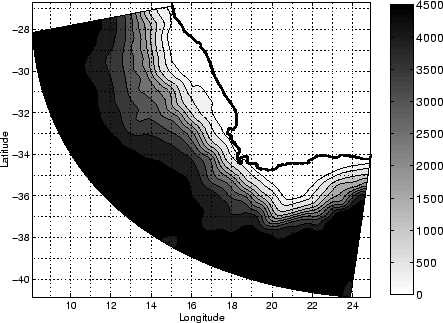 |
Figure 3.8:
Smoothed ocean topography (greyscale range in meters) for the low
resolution experiment.
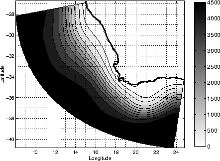 |
Comparing figure (3.6) and figure (3.7), one can note
that whereas some features like the Cape Canyon or the steep wall just South of the
Agulhas Bank have been filtered out, the major topographical characteristics remain
in the bathymetry used for the high resolution experiment. Although smaller, the
Agulhas Bank is approximately well represented as well as the widening of the shelf
in St. Helena Bay or the narrowing of the shelf South of Lüderitz. The filtering
has removed the narrow shelf in the Cape Peninsula area. For the low resolution
grid, most of the topographical features have been filtered out and there only remains a
very smoothed shelf break that follows the coastline. Tests have been conducted for
the high resolution configuration with a neutral stratification to validate the
value of the smoothing on the pressure gradient error.
On the vertical, we have chosen N=20 vertical levels. It would have been
interesting to use more vertical levels to resolve more accurately the bottom
layers, but tests along a vertical slice with an increased number of vertical levels
did not produce a significant improvement of the solution. The minimum depth has
been fixed at 30 meters and the maximum depth at 5000 meters. The number of levels
were concentrated at the surface where most of the variability occurs and to keep a
good resolution for the biological components (table 3.3.1 and figure
3.9). To do so, has been chosen equal 7, equal
0.3, and equal 20 meters. Note that with these parameter values, the
resolution is less than 5 meters everywhere at the surface, but can be really coarse
on the bottom of the deep ocean (more than 1000 m when h=5000 m) (table
3.3.1).
Table 3.1:
Vertical s-coordinate system: depth in meters of the s levels for the
w-points. The other variables are at intermediate levels.
| |
|
|
|
| Level |
at h |
at h |
at h |
| |
|
|
|
| 20 |
0.0 |
0.0 |
0.0 |
| 19 |
-1.0 |
-2.8 |
-4.7 |
| 18 |
-2.0 |
-6.5 |
-11.0 |
| 17 |
-3.0 |
-11.9 |
-20.7 |
| 16 |
-4.1 |
-20.5 |
-36.9 |
| 15 |
-5.1 |
-35.2 |
-65.2 |
| 14 |
-6.2 |
-61.1 |
-116.0 |
| 13 |
-7.4 |
-106.4 |
-205.5 |
| 12 |
-8.7 |
-181.7 |
-354.8 |
| 11 |
-10.1 |
-294.2 |
-578.3 |
| 10 |
-11.7 |
-436.9 |
-862.2 |
| 9 |
-13.3 |
-586.2 |
-1159.0 |
| 8 |
-14.8 |
-719.0 |
-1423.2 |
| 7 |
-16.3 |
-831.1 |
-1645.8 |
| 6 |
-17.7 |
-934.0 |
-1850.4 |
| 5 |
-19.1 |
-1045.7 |
-2072.2 |
| 4 |
-20.7 |
-1184.8 |
-2348.9 |
| 3 |
-22.4 |
-1371.8 |
-2721.2 |
| 2 |
-24.5 |
-1631.7 |
-3238.9 |
| 1 |
-26.9 |
-1997.5 |
-3968.1 |
| 0 |
-30.0 |
-2515.0 |
-5000.0 |
|
Figure 3.9:
Vertical s-coordinate system: vertical levels of the  points for a
section across the shelf North of St Helena Bay.
points for a
section across the shelf North of St Helena Bay.
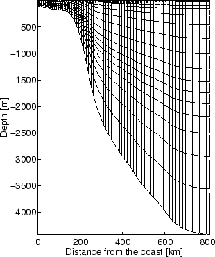 |
2 Surface fluxes
The atmospheric forcing fields are based on monthly climatologies derived from the
Comprehensive Ocean-Atmosphere Data Set (COADS) [Da Silva et al., 1994]. The momentum forcing
is given by the longitudinal and latitudinal components of the wind stress. One can
note on figure (3.10) that on the South Coast, the climatological wind
field in never favorable to upwelling. North of S the upwelling favorable
wind is perennial throughout the year, whereas it is seasonal South of S
[Shillington, 1998]. A cyclonic wind stress curl is present on the shelf associated with
the upwelling favorable wind.
Figure 3.10:
Wind
stress based on the COADS monthly climatology (1 vector is portrayed every 8
vectors). The greyscale range represent the wind stress curl ( ) in
N.m
) in
N.m .
.
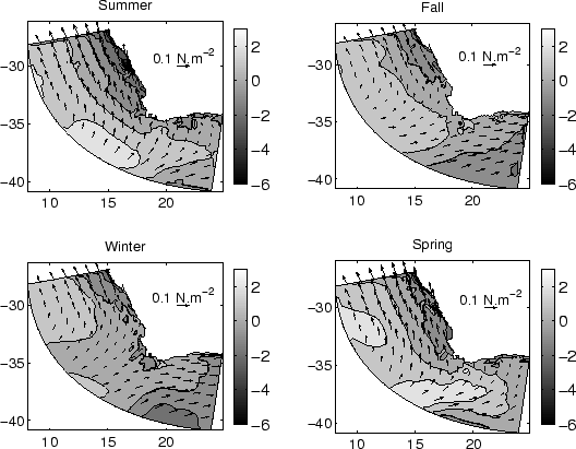 |
Figure 3.11:
Net heat
flux in W.m based on the COADS monthly climatology.
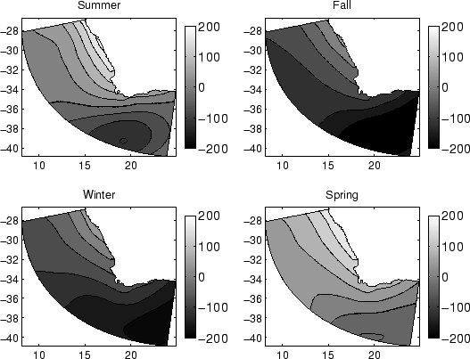 |
Setting up the thermohaline forcing of an ocean is less straightforward. The
specification of the surface fluxes alone may lead to an undesirable drift of the
model fields as it neglects the feed-back to the atmosphere entirely. Therefore,
basin scale models are often forced by nudging towards monthly mean climatological
surface fields. A method physically more satisfactory is to linearize the thermal
forcing around climatological sea surface temperature  , in order to
represent the model sea surface temperature
, in order to
represent the model sea surface temperature  feedback on the surface heat
fluxes [Barnier et al., 1998], as
feedback on the surface heat
fluxes [Barnier et al., 1998], as
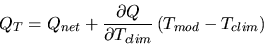 |
(93) |
The term
 is computed as
  from the
different contributions for the heat fluxes: infrared, sensible heat, and latent
heat [Siefridt, 1994]:
from the
different contributions for the heat fluxes: infrared, sensible heat, and latent
heat [Siefridt, 1994]:
 |
(94) |
Where is the constant of Stefan,  is the specific heat of the
atmosphere,
is the specific heat of the
atmosphere,  is the sensible heat transfer coefficient, is the wind speed,
 is the latent heat transfer coefficient, is the latent heat of
vaporization, and
is the latent heat transfer coefficient, is the latent heat of
vaporization, and  is the sea level specific humidity. The term
is portrayed on figure 3.12. For
a mixed layer depth of 50 m it corresponds to a nudging coefficient toward the
climatology ranging from about 50 days in the South to a maximum 90 days in the West
Coast. Figure (3.13) shows the sea surface temperature used for the
correction of the surface heat flux, obtained from the COADS dataset. In this dataset,
the Agulhas Current and the upwelling system are poorly represented.
is the sea level specific humidity. The term
is portrayed on figure 3.12. For
a mixed layer depth of 50 m it corresponds to a nudging coefficient toward the
climatology ranging from about 50 days in the South to a maximum 90 days in the West
Coast. Figure (3.13) shows the sea surface temperature used for the
correction of the surface heat flux, obtained from the COADS dataset. In this dataset,
the Agulhas Current and the upwelling system are poorly represented.
Figure 3.12:
Linear dependence of the net heat flux on the sea surface temperature in
W.m.C based on the COADS monthly climatology.
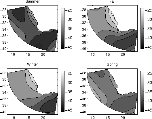 |
Figure 3.13:
Sea
surface temperature (C) of the COADS monthly climatology, used in the net heat
flux correction term.
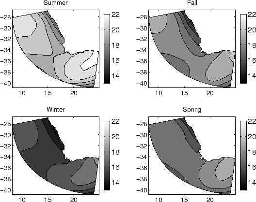 |
Figure 3.14:
Evaporation minus precipitation (cm.day) of the COADS monthly
climatology.
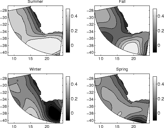 |
The fresh water fluxes are specified as salt fluxes based on the climatological
precipitation (P) and evaporation (E) fields (figure 3.14). The use of E-P
data independent of the model solution can induce a drift of the model solution
[Haidvogel et al., 2000]. To counter this behavior a correction term for the surface salinity
flux has been added to the formulation, identically to the heat flux correction
term. We obtain:
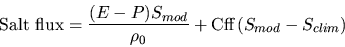 |
(95) |
This method has been chosen for our configuration, using a nudging
coefficient, corresponding to 75 days, the same order of magnitude as the
averaged value of the heat flux correction term. Unfortunately, a bug has crept
into the model and the salinity flux remained equal to zero during all the simulations.
Nevertheless, the cold water doesn't evaporate dramatically in an upwelling system
and the precipitation in the Benguela is low (figure 3.14). This induces
low values for the E-P field of the West Coast. The salinity fluxes coming from the
lateral boundaries should overwhelm the surface flux. Hence, we expect the solution
to not drift excessively from the climatology values.
3 Initial and boundary conditions
Coastal modeling requires well behaved, long term solutions for configurations with
open boundaries on up to 3 sides. A numerical boundary scheme should allow the
inner solution to radiate through the boundary without reflection and
information from the surrounding ocean to come into the model. The active open boundary
scheme implemented in ROMS estimates the two dimensional horizontal phase velocities
in the vicinity of the boundary [Marchesiello et al., 2000]. For each model variable ,
following Raymond and Kuo [1984], the normal ( ) and tangential(
 ) phase
velocities are:
) phase
velocities are:
If the propagation is towards the open ocean, the features produced inside the model
are evacuated following the wave equation:
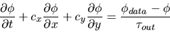 |
(98) |
If the propagation is towards the interior, the value at the boundary is nudged
towards data:
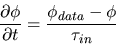 |
(99) |
The tangential and normal propagations are discretized in ROMS in an upstream biased
fashion, where the normal component is treated implicitly. Hence, this scheme
allows large time steps without loss of stability. At the corners the averaged
value of the two adjacent boundary points is taken. Mass conservation is
enforced around the model domain [Marchesiello et al., 2000]. The
inflow/outflow split scheme can cause problems in the sense that a grid point can be
an inflow for one process and an outflow for another (for example the Eastern boundary
is an inflow boundary for the Agulhas Current and the barotropic Rossby waves, but
it is an outflow boundary for coastal trapped waves and Kelvin waves). A series of
actions are taken to counter this problem in order to obtain a long term satisfactory
behavior of the solution:
- The solution is weakly relaxed
towards data in outflow conditions [right term of equation (3.36)].
- The solution is weakly nudged towards data in nudging bands close to the
boundaries. The nudging coefficient is linearly decreasing in the 6 points near the
boundaries (figure 3.15).
- Whereas no explicit mixing is mandatory
in the model domain, a sponge layer with linearly increasing lateral mixing
coefficient (figure 3.16) filters out the possible numerical noise or
reflections produced by the open boundaries. Recent simulations of the US West
Coast ocean model [Marchesiello et al., 2000] have shown that with the
active boundary condition schemes, the sponge layers were no longer necessary.
Figure 3.15:
Nudging time in days for the high resolution experiment.
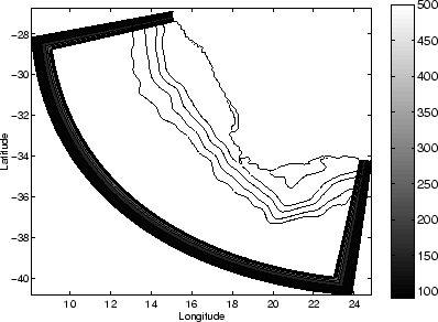 |
Figure 3.16:
Lateral
Laplacian mixing coefficient (m.s) for the high resolution experiment.
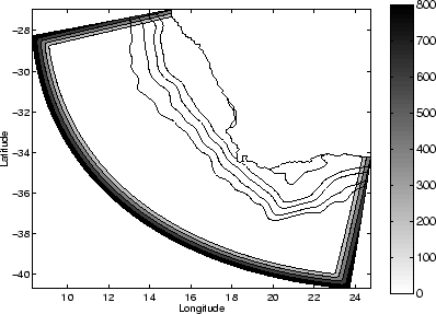 |
This method filters the model solution to connect it to the surrounding
smooth oceanic data, while allowing the development of a meaningful internal solution.
The relaxation times are chosen empirically to avoid long-term drift and
over-specification:
-
 days for all the
variables
days for all the
variables
 days for the velocities
 days
for the tracers
days
for the tracers
Since the boundary values of the free surface elevation does not affect the inner
solution on a C-grid, a simple non-gradient scheme is applied for the boundary
condition of the free surface elevation.
An important particularity of the regional model of the South African West Coast is
the highly energetic Agulhas Current that is flowing into the domain via the Eastern
boundary. In the presence of this meandering current, the solution happened to be instable after
a year or two of simulations. To obtain a long term stable solution, a specific open
boundary scheme has been implemented into the code for the barotropic component of
the velocities perpendicular to the boundaries. This scheme was originally proposed
by Flather [1976] for a tidal model, and combines a one dimensional radiation equation
(3.38) with a one dimensional version of the linearized continuity
equation (3.39):
 |
(103) |
The sign in equation (3.41) depends on the position of the boundary. For
the phase velocity, we assumes that the waves approaching the open boundary are
mostly non dispersive surface gravity waves. Hence, c in equation (3.41)
is fixed at  (g being the gravity acceleration and H the water column
depth). Equation (3.41) becomes;
(g being the gravity acceleration and H the water column
depth). Equation (3.41) becomes;
 |
(104) |
This open boundary scheme can be seen as a one way nesting scheme that conserves
mass. The differences between the specified values (
 and
and
 ), and those calculated by the model ( and ) are
forced to radiate at the speed of the external gravity waves [Palma and Matano, 1998].
Information is constantly provided by the boundary, that could over-determine the
inner solution. Nevertheless, if consistent data were provided for the boundary,
this scheme gave the best overall performance in test cases conducted using a
shallow water model [Palma and Matano, 1998]. One should expect that for a realistic simulation,
if data of good quality are given for the boundary, this scheme should stabilize the
inner solution in comparison to a scheme that allows a more important degree of
freedom. This is what it is observed during our simulation. The drawback is that an
important control from the boundaries could limit the physical significance of the
solution obtained inside the model domain.
In a first attempt, the initial and boundary conditions have been derived from a
global monthly climatology dataset [Levitus, 1982]. The sea surface elevation is
computed as the dynamic height referenced to the 500 m level. The thermal wind
relationship gave the baroclinic velocities. Several problems arose from this
derivation:
), and those calculated by the model ( and ) are
forced to radiate at the speed of the external gravity waves [Palma and Matano, 1998].
Information is constantly provided by the boundary, that could over-determine the
inner solution. Nevertheless, if consistent data were provided for the boundary,
this scheme gave the best overall performance in test cases conducted using a
shallow water model [Palma and Matano, 1998]. One should expect that for a realistic simulation,
if data of good quality are given for the boundary, this scheme should stabilize the
inner solution in comparison to a scheme that allows a more important degree of
freedom. This is what it is observed during our simulation. The drawback is that an
important control from the boundaries could limit the physical significance of the
solution obtained inside the model domain.
In a first attempt, the initial and boundary conditions have been derived from a
global monthly climatology dataset [Levitus, 1982]. The sea surface elevation is
computed as the dynamic height referenced to the 500 m level. The thermal wind
relationship gave the baroclinic velocities. Several problems arose from this
derivation:
- The solution was dependent of the arbitrary choice of the
no-motion reference level.
- Extrapolation was necessary to obtain data on the
shelf and gave spurious recirculation.
- The Agulhas Current was badly
represented (see figure 3.13).
Whereas it was possible to obtain a solution by this method, it has been preferred
to rely on a seasonal averaged data derived from a z-coordinate, 1/3
resolution, rigid lid, basin scale model of the Indian and South-Atlantic Oceans
[Biastoch and Krauß, 1999]. This model is currently implemented at the Oceanographic Department
of the University of Cape Town. The rigid lid assumption made in this model forces us to
diagnose a free surface elevation from the other variables. This seasonal data
gives an annual cyclic information for each model variable (e.g. u, v,
, , T, S, ). To avoid discontinuities in the climatology
(and forcing) fields, ROMS linearly interpolates in time the data to obtain a field
at each model time.
The summer values of the climatology (e.g. 15 February) are used for the initial
conditions. For the model spin-up, it has been preferred to let the model adjust
itself from rest on the density field associated with the temperature and salinity.
The variables u, v, , and are set to zero a t=0.
The circulation has
to adjust to the stratification, the domain geometry, the surface and the lateral
forcings. Because the domain is relatively small, this should occur relatively
quickly, and we expect to obtain an equilibrium state after a few years of
simulation.
4 Results for the low resolution model
1 Spin-up
Figure 3.17:
Sea
surface height and barotropic currents for the low resolution experiment. a: after
1 day of simulation. b: after 1 week. c: after 2 weeks. d: after 1 month. The
greyscale range represents the sea surface elevation in centimeters. 1 current
vector is portrayed every 4 vectors.
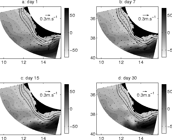 |
As explained by Penduff [1998], several mechanisms rapidly adjust the solution to
the initial stratification, and the different forcing. After 1 day, the sea surface
elevation shows the geostrophic adjustment to the initial stratification (figure
3.17-a), . From the Northern boundary, a signal of low elevation
(associated with the upwelling) propagates along the West Coast to the South as a
coastal trapped wave (figures 3.17-a, 3.17-b
and 3.17-c), and
connects with locally forced low sea surface elevation around Cape Peninsula. The
adjustment processes induce relatively strong barotropic velocities on the Agulhas
Bank (figures 3.17-a and 3.17-b). After 15 days, the
velocities are weaker on the shelf and slope (figure 3.17-c), and a ring
detaches from the Agulhas Current.
Figure 3.18:
Sea surface height and barotropic currents for the low resolution
experiment. a: 3 January of model year 2. b: 3 January of model year 5. c: 3
January of model year 10. d: 3 January of model year 15. The greyscale range
represents the sea surface elevation in centimeters. 1 current vector is portrayed
every 4 vectors.
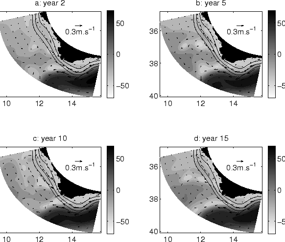 |
Figure 3.19:
Root
mean square of the sea surface elevation over the domain
The thick line represents the data after a low pass filter with a cutoff at 1 year.
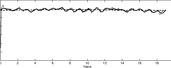 |
Though the model resolution is coarse (ranging from 18 km to 31 km), mesoscale
activity is able to develop during the simulation. On figure (3.18),
the sea surface elevation and the barotropic currents have been portrayed for 3
January of model year 2 (figure 3.18-a), model year 5 (figure
3.18-b), model year 10 (figure 3.18-c), and model year
15(figure 3.18-d). After 1 year of simulation (figure
3.18-a), the solution appears to be adjusted. Regardless of the
mesoscale activity, very few differences occur in the following years. Cyclonic
eddies appears to be shed from the Agulhas Bank and from the Cape Point / Cape
Columbine area. Though very close to the open boundary, from time to time an
anticyclonic eddy detaches from the Agulhas Current at the Agulhas retroflection
(figure 3.18-b). The adjustment process can be seen on a graph of the
domain averaged norm of :
 (figure: 3.19). The model "forgets" quasi immediately the shock
of the start from rest. A low pass filtering with a cut-off at 1 year is applied to
the data (thick line on figure 3.19) to show the seasonal and
interannual variability. No significant long term trend is observed after the first
adjustment of the sea surface elevation.
(figure: 3.19). The model "forgets" quasi immediately the shock
of the start from rest. A low pass filtering with a cut-off at 1 year is applied to
the data (thick line on figure 3.19) to show the seasonal and
interannual variability. No significant long term trend is observed after the first
adjustment of the sea surface elevation.
Figure 3.20:
Volume averaged potential temperature ( C)for the low resolution
experiment as a function of time.The thick line represents the data filtered by a
low pass filter with a cut off at 4 years. The dotted line
represents the trend of the data.
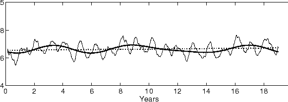 |
Figure 3.21:
Volume averaged salinity (PSU) for the low resolution experiment as a
function of time. The thick line represents the data filtered by a low pass filter
with a cut off at 4 years. The dotted line represents the trend of the
data..
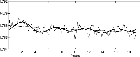 |
After the quick adjustment to the initial values, the slow response of the
stratification occurs. These long term processes consist of the propagation of
baroclinic waves, advection and mixing. The presence of the Agulhas Current
associated with strong velocities accelerates the adjustment process. Because the
domain is relatively small, it takes a relatively short time for a baroclinic wave
or an advected water particle to cross it. An important measure of model fidelity
is the degree to which it is able to preserve the globally averaged values of its
tracer fields. The volume averaged temperature time series shows a strong seasonal
pattern (figure 3.20). After 2-3 years it oscillates around a
mean of approximately  C. No significant trend is noticeable. But the
solution exhibits variations on the interannual scale. This variability
is quite surprising. It can be related to the presence of the Agulhas Current that
produces, on an irregular basis, large eddies in comparison with the size of the
domain. Interannual variability is also a characteristic pattern observed in the
time series of the domain averaged salinity (figure 3.21).
Freshening occurs during the 5 first years, in a range of 0.002 PSU. As the surface
forcing didn't operate correctly during this simulation, a trend should have been
noticed in the volume averaged salinity. The weakness of the observed trend
emphasises an important constraint of the open boundaries on the solution. Tests
should be conducted with less restrictive open boundary nesting values.
C. No significant trend is noticeable. But the
solution exhibits variations on the interannual scale. This variability
is quite surprising. It can be related to the presence of the Agulhas Current that
produces, on an irregular basis, large eddies in comparison with the size of the
domain. Interannual variability is also a characteristic pattern observed in the
time series of the domain averaged salinity (figure 3.21).
Freshening occurs during the 5 first years, in a range of 0.002 PSU. As the surface
forcing didn't operate correctly during this simulation, a trend should have been
noticed in the volume averaged salinity. The weakness of the observed trend
emphasises an important constraint of the open boundaries on the solution. Tests
should be conducted with less restrictive open boundary nesting values.
Figure 3.22:
Top:
Volume averaged kinetic energy (cm.s) for the low resolution experiment.
Bottom: Surface kinetic energy (cm.s) for the low resolution
experiment.
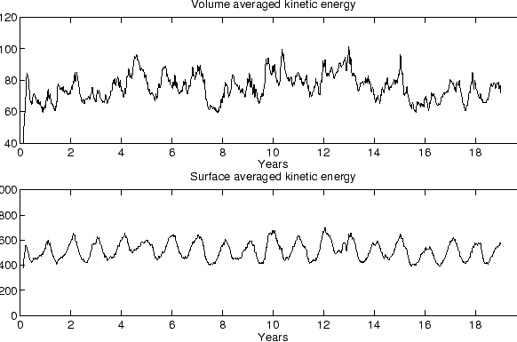 |
Time series of the volume averaged kinetic energy and of the averaged surface
kinetic energy are shown on figure (3.22-top) and figure
(3.22-bottom) respectively.
During the first months of the simulation, the
volume averaged kinetic energy rises rapidly to reach an averaged value of about 90
cm.s. Little temporal trend is apparent in the time series. The
seasonal pattern is not really dominant in the volume averaged kinetic energy. On
the contrary, the surface kinetic energy shows the marked ocean response to the
seasonal varying surface forcing. The absence of a significant trend is a sign of
correct behavior of the solution. As expected, the surface averaged kinetic energy
has a maximum during the upwelling season.
2 Time average
The outputs of the low resolution experiment have been time averaged from model year
3 to model year 10 in order to obtain a smooth 3-dimentional field of the mean
circulation resolved by the model.
Figure 3.23:
Annual surface climatology derived from the results of the low resolution
experiment. a: sea surface temperature (C). b: surface currents
(m.s), Vmax is the maximum velocity, 1 vector is portrayed every 4 vectors.
c: sea surface salinity (PSU). d: sea surface height (m). The horizontal
coordinates account for the longitude and the latitude.
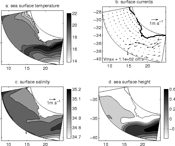 |
For the low resolution experiment, the averaged sea surface temperature is close to
the surface climatology employed for the heat forcing of the model (figure
3.23-a). Upwelling is relatively homogeneous with 14C waters
all along the west coast from Cape Peninsula to the northern boundary. The
isotherms tend to move away from the coast North of 30 S, but the northern
boundary constrains them back towards the coast north of 29 S. The Agulhas
current is characterized by a tongue of warm water ( C) that rounds the
Agulhas Bank, enclosing colder surface water onto the bank. The presence of the
Subtropical front is noticeable in the South Corner of the model domain. It shows a
marked sea surface temperature gradient ranging form 13C to 17C in
a short distance. The Agulhas Current does not retroflect properly in
this experiment (figure 3.23-b). When it flows along the Agulhas
Bank, it reaches on average a maximum velocity of 1.1 m.s, which is a
realistic value. Because the topography is smooth, the current does not detach from
the southern tip of the Agulhas Bank, and rounds the bank to flow in a North-east
direction. This behavior is not observed in nature. As a consequence, the
retroflexion area is displaced westward close to the offshore boundary. On the
Agulhas Bank, currents are weak as pointed by Boyd and Oberlholster [1994]. The
Good Hope jet is not present on the western part of the bank. Along the west coast,
the north westward surface current flows continuously towards the equator with
characteristic velocities of about 30 cm.s. Divergence is evident offshore
of Cape Columbine (17 E - 33 S), in agreement with the schematic
representations of Boyd and Shillington [1994] (figure 1.8) and Shannon
[1985] (figure 1.13). The Subtropical front is well represented by
the surface salinity (figure 3.23-c) with values ranging from 34.6
PSU to 35 PSU in the South corner of the model domain. The effect of the zero
surface salinity flux is visible near the northern boundary where the solution has
departed from the climatology forcing values and is restored back in the vicinity of the
boundary. Nevertheless, the averaged surface salinity values remain close (in a
range of
C) that rounds the
Agulhas Bank, enclosing colder surface water onto the bank. The presence of the
Subtropical front is noticeable in the South Corner of the model domain. It shows a
marked sea surface temperature gradient ranging form 13C to 17C in
a short distance. The Agulhas Current does not retroflect properly in
this experiment (figure 3.23-b). When it flows along the Agulhas
Bank, it reaches on average a maximum velocity of 1.1 m.s, which is a
realistic value. Because the topography is smooth, the current does not detach from
the southern tip of the Agulhas Bank, and rounds the bank to flow in a North-east
direction. This behavior is not observed in nature. As a consequence, the
retroflexion area is displaced westward close to the offshore boundary. On the
Agulhas Bank, currents are weak as pointed by Boyd and Oberlholster [1994]. The
Good Hope jet is not present on the western part of the bank. Along the west coast,
the north westward surface current flows continuously towards the equator with
characteristic velocities of about 30 cm.s. Divergence is evident offshore
of Cape Columbine (17 E - 33 S), in agreement with the schematic
representations of Boyd and Shillington [1994] (figure 1.8) and Shannon
[1985] (figure 1.13). The Subtropical front is well represented by
the surface salinity (figure 3.23-c) with values ranging from 34.6
PSU to 35 PSU in the South corner of the model domain. The effect of the zero
surface salinity flux is visible near the northern boundary where the solution has
departed from the climatology forcing values and is restored back in the vicinity of the
boundary. Nevertheless, the averaged surface salinity values remain close (in a
range of  PSU) to the Levitus [1982] climatology data. The Agulhas
Current does not have a marked signature in surface salinity. On the contrary, it
dominates the averaged sea surface elevation signal 3.23-d). In
the few kilometers between the Agulhas Bank and the southern part of the Agulhas
Current, the averaged sea surface elevation ranges from -30 cm to 60 cm (figure
3.23-d). Along the west coast, the variations in sea surface
height are very small (
PSU) to the Levitus [1982] climatology data. The Agulhas
Current does not have a marked signature in surface salinity. On the contrary, it
dominates the averaged sea surface elevation signal 3.23-d). In
the few kilometers between the Agulhas Bank and the southern part of the Agulhas
Current, the averaged sea surface elevation ranges from -30 cm to 60 cm (figure
3.23-d). Along the west coast, the variations in sea surface
height are very small ( cm).
cm).
Figure 3.24:
Averaged currents in m.s for the low resolution experiment. a: for
 m, b: for
  m, c: for
  m, and d: for
  m. The
maximum velocity is given for each level. One vector is represented every 4
vectors. The horizontal coordinates account for the longitude and the latitude.
m. The
maximum velocity is given for each level. One vector is represented every 4
vectors. The horizontal coordinates account for the longitude and the latitude.
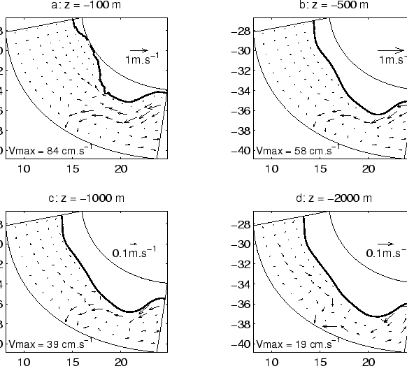 |
The horizontal averaged currents have been portrayed for z = -100 m (figure
3.24-a), z = -500 m (figure 3.24-b), z = -1000 m
(figure 3.24-c), and z = -2000 m (figure 3.24-d).
The Agulhas current is present on the 3 first levels. Its magnitude diminishes
smoothly with depth. For z=-100 m (figure 3.24-a), a narrow
coastal jet with velocities of 30 cm.s flows past Cape Peninsula towards the
equator. Between this jet and the coast, the equatorward flow is weak. For z=-500 m
(figure 3.24-b), poleward motion is present along the topography
North of 32 S. Between Cape Peninsula and 32 S equatorward motion is still
present. Below 500 m weak poleward motion is present North of 36 S (figures
3.24-c and 3.24-d) as described by Nelson [1989].
Figure 3.25:
Potential temperature annual climatology (C) for the low resolution
experiment. a: for m, b: for m, c: for m, and d:
for m. The horizontal coordinates account for the longitude and the
latitude.
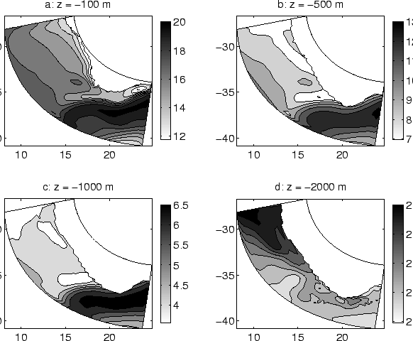 |
Figure 3.26:
Salinity annual climatology (PSU) for the low resolution experiment. a:
for m, b: for m, c: for m, and d: for m.
The horizontal coordinates account for the longitude and the latitude.
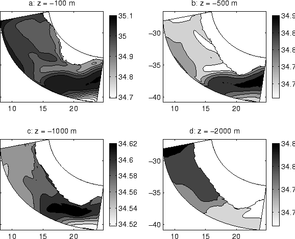 |
The potential temperature and the salinity have been also portrayed for the 4
horizontal levels defined previously (figures 3.25 and
3.26). The upwelling signal all along the west coast is present
for z=-100m with a minimum in temperature (12 C, figure 3.25-a)
and a minimum in salinity (34.7 PSU, figure 3.26-a). This minimum
in salinity is caused by the presence of the Antarctic Intermediate Water (AAIW),
characteristic of the South-East Atlantic Ocean, with its core of minimum of salinity
around 700-800 m (see section 1.2). This minimum of salinity can
diminish the density gradient induced by the upwelling in comparison to the other
upwelling systems. This is a particularity of the Benguela. The impact of this
salinity minimum on the dynamics of the upwelling system still have to be
quantified. On the eastern side of the Agulhas Bank, for z = -100 m, a local
minimum in temperature stands at the offshore limit of the shelf. It can be the
signature of the subsurface cool-water feature described by Boyd and Shillington
[1994]. For z = -100 m, -500 m, and -1000 m, the Agulhas Current is recognizable by
a maximum both in salinity and temperature. At these levels, a zonal tongue of
local minimum of temperature and salinity extends from the Agulhas Bank at 35 S.
An averaged cyclonic circulation of the surface currents (visible also in the sea
surface elevation) is associated to this structure. It might be related to upwelled
waters transported offshore by mesoscale eddies shed from the Agulhas Bank-Cape
Peninsula area. For z = -2000 m, an equatorward increase of potential temperature
of 0.4 C (figure 3.25-d) and for salinity of 0.15 PSU (figure
3.26-d) over the length of the domain is visible. This shows a
transition from Antarctic Intermediate Water to North Atlantic Deep Waters (see the
TS-diagram 1.4).
Although the results of the low resolution experiment show interesting features that
can be related to observations, some aspects of the solution, like the Agulhas
Current retroflection or the coastal circulation, are not well represented at this
level of resolution. The bottom topography appears to have an important control of
the flow and need to be treated more accurately. Hence, a new set of experiments is
conducted by doubling the horizontal number of grid points in each direction.
Nevertheless, the low resolution configuration is a useful tool that provides a
reference solution to compare with new results and that can be used to test new
numerical schemes or parameterizations at a reasonable computer cpu time.
5 Results for the high resolution model
Keeping the same surface and lateral boundary forcing of the previous experiment, a
new configuration has been set up using an horizontal grid with an accuracy ranging
from 9 km at the coast to 16 km offshore. This configuration should resolve most
of the mesoscale features observed along the southwestern coast of Africa. The
criterion for the error in the pressure gradient allows the use of a less smoothed
bottom topography (figure 3.7). Because the bathymetry is of primary
importance in the control of the shelf and slopes dynamics, the behavior of the
solution in this configuration should be more satisfactory.
Figure 3.27:
Left panel: bottom layer currents (cm.s) after 1 month for the
sigma coordinate test case in high resolution. The greyscale range represents the
total velocity in cm.s. The isolines interval is 1 cm.s.The
horizontal coordinates account for the longitude and the latitude. Right panel:
maximum current (cm.s) over all the domain as a function of time in days.
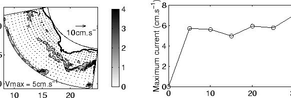 |
In a first step, the effects of the s-coordinate related pressure gradient error are
tested in an experiment with no forcing and no horizontal variations in density.
Four walls are placed at the lateral boundaries of the domain. The vertical
structures in temperature and salinity are defined analytically at the model
initialization to account for the horizontally spatial average of the vertical
density structure. During this test, no horizontal or vertical mixing is present,
to concentrate on the effects of the pressure gradient. Because there is no forcing
and no horizontal variations in density, the pressure gradient should remain equal
zero during all the simulation. If currents are generated, they are spurious
circulations induced by errors in computing the pressure gradient. The spurious
circulation should be maximum in the bottom s-level, where the slopes in the s
coordinates are the highest. As explained in section (3.2.4), the
s-coordinate related pressure gradient error comes from the discretization of the
pressure gradient in the s-coordinate system. If the density field and the
s-coordinate system do not vary with time, the error in the pressure gradient
should remain constant for this test case (the s-coordinate is dependent of the free
surface elevation but this only significantly affects the surface layers). Because
only the Coriolis and pressure gradient terms are solved during the test simulation,
the spurious currents should reach rapidly a geostrophic equilibrium with the error
in the pressure gradient. Hence, after a spin-up of a few days, the averaged
spurious currents should not increase with time. It is then sufficient to run the
test experiment for only a month to obtain a significant representation of the
impact of the pressure gradient error on the circulation. During the test
experiment, the maximum spurious currents reach a plateau of about 6 cm.s
after 5 days (figure 3.27-right). It is a large value but
looking at the horizontal currents of the s-bottom level after 1 month of simulation
(figure 3.27-left), one might note that this largest currents are
along the domain wall (that are open boundaries in the realistic experiment).
Hence, these currents are not directly forced by errors in the pressure gradient,
but are part of the general circulation generated to compensate the slow motion
induced by the pressure gradient errors. At distance from the walls, the bottom
spurious currents are of the order of 1 cm.s with a maximum of 2 cm.s
South of the Agulhas Bank (figure 3.27-left). The
pressure-gradient-error-related-currents are portrayed after 1 month of simulation
at 4 horizontal levels: z = -100 m (figure 3.28-a), z =
-500 m (figure 3.28-b), z = -1000 m (figure
3.28-c), and z = -2000 m (figure
3.28-d). At each level, the error results in a poleward
along-slope current of around 1 to 2 cm.s. The current is locally stronger
( 5 cm.s) at the southern tip of the Agulhas Bank for z = -1000 m. If
we compare the error induced currents to the time averaged currents of the high
resolution realistic experiment (figure 3.33), we can note that the
relative error is of approximately 5 % for z = -100 m, 10 % for z = -500 m , and
20 % for z = -1000 m and z = -2000 m. These values are not small for the deep
layers. A part of the solution can be induced by errors in the pressure gradient.
This might be the case for the deep poleward motion observed in figure
(3.33-d) and for the poleward undercurrent observed on figure
(3.45-b). One can note firstly that the values obtained for
these 2 currents corresponds to observation [Nelson, 1989]. Secondly the residual
pressure gradient related current obtained in the test case are of the same order of
magnitude of the error made in the measurements. Thirdly, the current pathway
observed on figure (3.33-d) is not the same as the pathway
followed by the error related current seen in figure (3.28-d).
Figure 3.28:
Horizontal currents in cm.s after 1 month for the test of the
pressure gradient error. a: for m, b: for m, c: for
m, and d: for m. One vector is represented every 4 vectors. The
horizontal coordinates account for the longitude and the latitude.
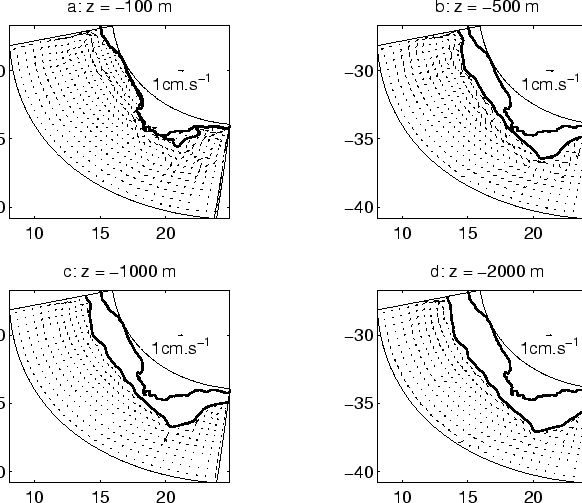 |
The realistic simulation in high resolution has been conducted for 10 years. The
data for the different modelized variables have been stored in an output file every
2 simulated days. This way, analysis of the model outputs are conducted with a high
level of spatial and temporal accuracy. These data are also employed to force an
individual based model developed at the University of Cape Town to study the
behavior of the eggs, larvae, and juveniles of sardines and anchovies around the
south and west coast of Africa. Like for the low resolution experiment, the spin up for
the high resolution experiment occurs quickly. After 1 year of
simulation, the solution appears to be already adjusted to the different forcing.
A high level of mesoscale activity develops during the simulation, activity
characterized by the generation of Agulhas rings from the Agulhas Current
retroflection area, the shedding of cyclonic eddies form the southern tip of the
Agulhas Bank, Cape Peninsula, and Cape Columbine. The upwelling front shows also an
important variability, developing a series of meanders, plumes and filaments in a
realistic manner. In the following sections, an analysis of the averaged behavior
of the model solution and variability as well as comparisons with observations
validate the simulation.
Figure 3.29:
Volume averaged potential temperature (C) for the high resolution
experiment as a function of time in years.The thick line represents the data
filtered by a low pass filter with a cut off at 4 years. The dotted line
represents the trend of the data.
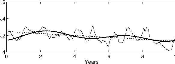 |
Figure 3.30:
Volume averaged salinity (PSU) for the high resolution experiment as a
function of time in years. The thick line represents the data filtered by a low
pass filter with a cut off at 4 years. The dotted line represents the
trend of the data.
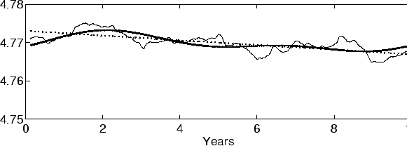 |
As for the low resolution experiment, time series are shown
of the volume averaged potential
temperature and salinity are portrayed respectively on figure
(3.29) and on figure (3.30).
The spin up appears to be as quick as for the low
resolution experiment. The volume averaged temperature shows seasonal variations
and a trend of -0.1C in 10 years (figure 3.29). A surprising
result is the trend observed in the time series of the volume averaged salinity, 10
times greater than for the low resolution experiment (nevertheless it is still
small). This exhibits the weaker influence of the open boundaries on the
inner solution. Two important events are visible as minimums both in the temperature
and salinity time series, at year 6 and after year 9. These minimums correspond
to a bifurcation in the pathway of the Agulhas Current associated with a large
cyclonic eddy perturbing the solution close to the Agulhas Bank. During the two
events, the retroflection area has moved towards the eastern boundary of the domain.
These variations in the position of the retroflection of the Agulhas Current have
been observed in nature.
Figure 3.31:
Top:
Volume averaged kinetic energy (cm.s) for the high resolution experiment.
Bottom: Surface kinetic energy (cm.s) for the high resolution
experiment.
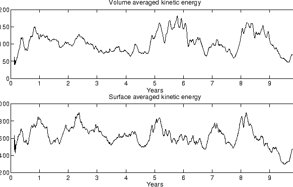 |
Because smaller structures are resolved in the high resolution experiment, the
volume averaged kinetic energy has increased from a mean value of 70 cm.s
to 100 cm.s with increasing resolution (figure
3.31-top). The 2 events described previously are also visible as
maximums in kinetic energy from year 5 to year 6 and from year 8 to year 9. The
seasonal pattern in the mean surface kinetic energy is less marked than for the low
resolution experiment. This reveals that more intrinsic instability processes,
not directly forced by the wind, are now resolved during the high resolution
experiment (figure 3.31-bottom). The mean level of surface kinetic
energy is also greater (600 cm.s) in the high resolution experiment than
for the low resolution experiment (500 cm.s).
1 Time averaged variables
By taking the average in time of the different model variables from year 3 to year
10, it has been possible to verify the improvement of the model solution when the
resolution has been increased.
Figure 3.32:
Annual surface climatology derived from the results of the high resolution
experiment. a: sea surface temperature (C). b: surface currents
(m.s), Vmax is the maximum velocity, 1 vector is portrayed every 4 vectors.
c: sea surface salinity (PSU). d: sea surface height (m). The horizontal
coordinates account for the longitude and the latitude.
 |
For the sea surface temperature (figure 3.32-a), the pathway of
the sea surface temperature signature Agulhas Current differs slightly from the low
resolution experiment. It no longer rounds the Southern limit of the Agulhas Bank
in an unrealistic way. The averaged position of the retroflection area is visible
in the image of averaged surface current and sea surface elevation (figures
3.32-b and 3.32-d). Some wave like meanders in
the upwelling front along the west coast are noticeable in figure
(3.32-a), and a jet that follows the shelf edge is present between
the southern tip of the Agulhas Bank and Cape Peninsula (figure
3.32-b) as observed in ADCP current measurements [Boyd and Oberholster, 1994].
These specific features of the coastal dynamics of the west coast are subject to a
more detailed analysis further in the manuscript. Few differences are
noticeable between the low and high resolution experiments for the averaged sea
surface salinity (figure 3.32-c).
Figure 3.33:
Averaged currents in m.s for the high resolution experiment. a:
for m, b: for m, c: for m, and d: for m.
The maximum velocity is given for each level. One vector is represented every 6
vectors. The horizontal coordinates account for the longitude and the latitude.
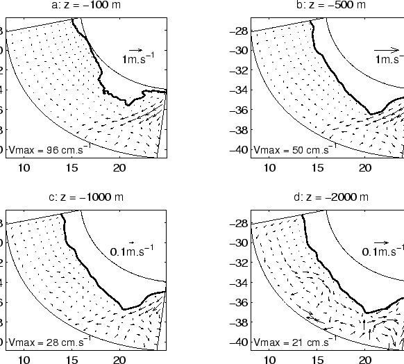 |
The time averaged horizontal currents are portrayed for z = -100 m, -500 m, -1000 m,
and -2000 m (figure 3.33). The Agulhas Current and the
retroflection are present in the 3 first levels. At these 3 levels an anticyclonic
recirculation is noticeable where the Agulhas Current encounter the western open
boundary. This might be related to an average position for the Agulhas Rings that
are shed from the Agulhas retroflection throughout the simulation. Coastal currents
along the west coast are equatorward for z = -100 m. For the lowers levels, the
currents along the topography appears to be very weak. In the wide area between the
coast and the offshore open boundary the eastern limb of the South Atlantic
subtropical gyre manifest itself by a meandering equatorward mean current visible
for z = -100 m and z = -500 m. At deeper levels, current in this area appears to be
more convoluted and a mean offshore poleward flow is present for z = -2000 m, as in
the low resolution experiment.
Figure 3.34:
Potential temperature annual climatology (C) for the high resolution
experiment. a: for m, b: for m, c: for m, and d:
for m. The horizontal coordinates account for the longitude and the
latitude.
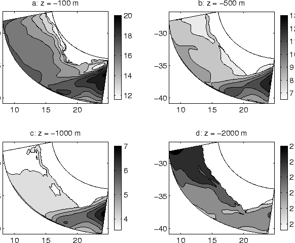 |
Figure 3.35:
Salinity annual climatology (PSU) for the high resolution experiment. a:
for m, b: for m, c: for m, and d: for m.
The horizontal coordinates account for the longitude and the latitude.
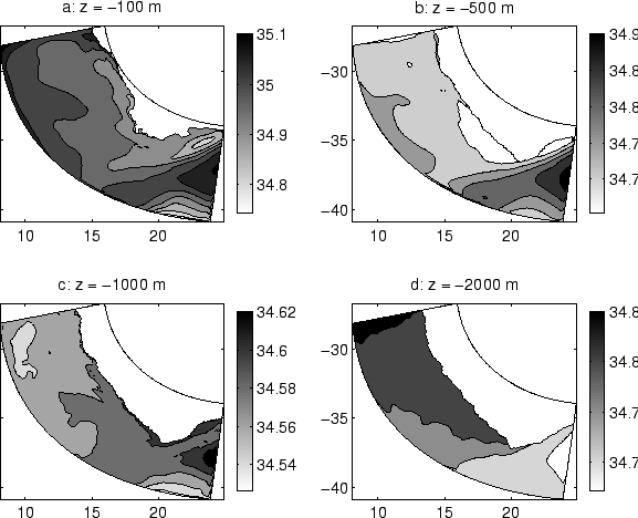 |
On the large scale, few differences appear in the comparison between the low and
high resolution experiments for the average potential temperature (figures
3.25 and 3.34) and the average salinity (figures
3.26 and 3.35). For the high resolution
experiment, the retroflection of the Agulhas Current is visible for temperature and
salinity for z = -100 m, -500 m, and -1000 m. The low temperature and salinity
tongue, described in section (3.4.2) extending from the Agulhas Bank is
no longer present for z= - 500 m and -1000 m. This feature should be related to the
smoothed topography of the low resolution experiment. For z = -100 m the subsurface
cool water feature on the eastern part of the Agulhas Bank described previously is
more marked in this simulation (figure 3.34-a) and can be seen
also in salinity. For z = -500 m, a narrow band of warmer water of unknown origin
is present along the shelf edge in the northern part of the domain.
Figure 3.36:
Transport stream function (Sv) derived from annual climatology of the high
resolution experiment. The isocontour interval is 10 Sv. The horizontal
coordinates account for the longitude and the latitude.
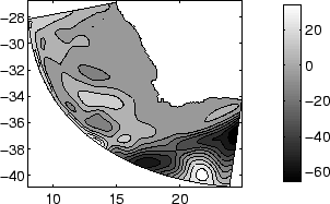 |
If we note  ,
,  and
and  the time averaged barotropic
velocities and free surface elevation, and if we remark that the free surface
elevation is small compare to the depth of the ocean depth , the time averaged
vertical integrated equation of continuity takes the form:
the time averaged barotropic
velocities and free surface elevation, and if we remark that the free surface
elevation is small compare to the depth of the ocean depth , the time averaged
vertical integrated equation of continuity takes the form:
Hence, the time averaged transport is
non-divergent and a time averaged transport function can be extracted from the time
averaged barotropic velocities. The resulting time averaged transport function for
the high resolution experiment is portrayed on figure (3.36). It
shows that the averaged transport associated with the Agulhas Current is around 65
Sv, and that the averaged transport of the simulated part of the Benguela ranges
from 10 Sv to 20 Sv. These values can be compared to the measured transport of 75
Sv for the Agulhas Current and of 15 Sv for the a similar part of the Benguela
current (figure 1.5) [Shannon and Nelson, 1996].
2 Comparison with temperature and salinity data
Figure 3.37:
a: sea surface temperature for the high resolution experiment for the
summer months. b: sea surface temperature for the high resolution experiment for
the winter months. c: sea surface temperature from the pathfinder satellite data
set for the summer months. d: sea surface temperature for the from the pathfinder
satellite data set for the winter months. The interval between the isotherms is
1C.
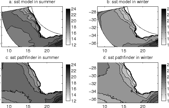 |
Though the linear parameterization of the sea surface temperature feedback on the
sea surface heat fluxes can be seen as a restoring term toward climatological sea
surface temperature data, it makes sense to compare the averaged sea surface
temperature generated by the model to more accurate data than the ones employed to
force the model. In figure (3.37), the model sea surface
temperature is compared to sea surface temperature measured from 1987 to 1999 by
satellite Pathfinder with an accuracy of 9 km. To make the comparison possible,
satellite and model data are averaged separately in the austral winter months (from
April to September) and in the austral summer months (from October to March). It
can firstly be noticed that the seasonal sea surface temperature patterns obtained
from the high resolution simulation differ from the smooth climatology used to
force the model (figure 3.13), whereas it compares remarkably to the
Pathfinder averaged data (figure 3.37), denoting a good behavior of
simulated smaller scale structures. For the summer months, one can note on the
panel (3.37-a) that the upwelling starts from Cape Agulhas with
identical values in the Pathfinder dataset (figure 3.37-c). The
temperature in a very narrow band close to the coast around 32 S is 3C to
4C smaller in the simulated field (figure 3.37-a) than in the
observation (figure 3.37-c). This can be related to the wind forcing
which is too large close to the coast and/or to a small inaccuracy in the satellite
measurement of the sea surface temperature close to the west coast. The summer
pathway of the modeled 18C isotherm that detaches from Cape Columbine to come
back to the coast 150 km downstream along the coast (figure 3.37-a)
is identical, between 35 S and 31 S, to the pathway of the 17C isotherm
in satellite data (figure 3.37-c). Further North, in summer, the
modeled isotherm tends to move off-shore to come back towards the coast near the
northern open boundary. This behavior is not observable on satellite data. A
little bump in the 20C isotherm is present at the southern tip of the Agulhas
Bank both in the model and satellite data for the summer months (figures
3.37-a and 3.37-c). It is the signature of the
shelf edge equatorward current flowing from the southern tip of the Agulhas Bank
towards Cape Peninsula. On the eastern part of the Agulhas Bank, a reverse plume is
present in model data, whereas only a bend in the Agulhas Current is visible on
satellite sea surface temperature data. For the winter months, the model solution
(figure 3.37-b) is also close to the pathfinder sea surface
temperature data (figure 3.37-d). Particularly, the cooling of
surface waters on the inner Agulhas Bank and the standing wave pattern (with a wave
length of about 150 km) just North of St Helena Bay can be observed in both
portrayals (figures 3.37-b and 3.37-d).
Figure 3.38:
a:
average sea-bottom temperatures (C) over the continental margin off
south-western Africa. b: average sea-bottom salinities (PSU) over the continental
margin off south-western Africa. Adapted from Dingle and Nelson [1993].
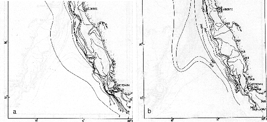 |
Figure 3.39:
a:
simulated climatological bottom temperatures (C) . b: simulated climatological
bottom salinities (PSU).
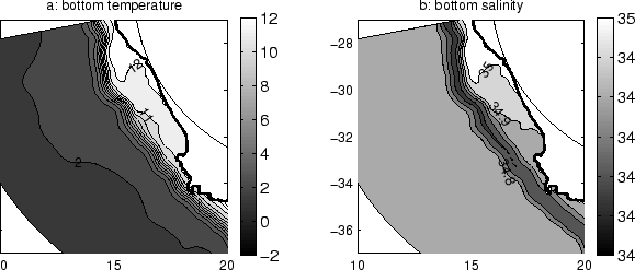 |
Dingle and Nelson [1993] have extracted the temporal average of a large amount of
temperature and salinity data for the bottom of the ocean along the west coast of
South Africa (figure 3.38). The first level of the s-coordinate follows
the bottom of the ocean. Hence, it is straightforward to extract averaged values
for the simulated sea bottom temperature and salinity (figure 3.39) to
compare to observations. The model bottom temperatures on the abyssal plain
(2C) and on the slope along the west coast (figure 3.39-a) are
identical to the observed ones (figure 3.38-a). On the shelf, the model
bottom temperature is warmer ( 11-12 C) than the observations ( 9-10
C), this difference can be a consequence of the absence of a parameterization of
the bottom mixed layer during the simulations. Because river runoffs are not taken
into account during the simulation, the warm signature of the Orange River outflow,
noticeable on figure (3.38-a), is not visible on the model outputs. The
invasion of colder water on the shelf from the South, described by Dingle and Nelson
[1993], is visible both in the model and the observations. The same remarks can be
made for the salinity with bottom shelf waters saltier ( 34.8-35 PSU, figure
3.39-b) than in the observations ( 34.7-34.9 PSU, figure
3.38-b). The minimum of salinity due to the Antarctic Intermediate
Water, observed along the slope (34.4 PSU, figure 3.38-b), is a bit
smaller than the minimum visible in the outputs of the model (34.6 PSU, figure
3.39-b). This difference can be due to the data employed at the model
initialization and in the forcing of the model open boundaries.
These model-data comparisons show a correct behavior of the time averaged
model solution. The analysis has now to be extended to check if the variability of
the modelized circulation compares also to the observations. This is done in the
next section.
3 Variability
The previous section was focusing on the time average model variables ( ). In
this section we will concentrate on the anomalies departing from the time averaged
variables (
). In
this section we will concentrate on the anomalies departing from the time averaged
variables ( ). By definition, the time average of the anomalies is zero,
thus we will concentrate on the variance of the anomalies (
). By definition, the time average of the anomalies is zero,
thus we will concentrate on the variance of the anomalies ( ). The standard
deviation, or root mean square, can be obtained by taking the square root of the
variance (
). The standard
deviation, or root mean square, can be obtained by taking the square root of the
variance ( ). It is an indicator of the variability produced during
the simulations.
). It is an indicator of the variability produced during
the simulations.
Figure 3.40:
Root mean
square of the sea surface temperature anomaly (C). top: from the high resolution
experiment. b: from monthly Pathfinder (1987-1999) satellite data. The interval
between the isocontours is 0.1 C. The horizontal coordinates account for the
longitude and the latitude
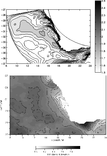 |
The root mean square of the sea surface temperature is portrayed on figure
(3.40-top) for the model results from year 3 to year 10 and on figure
(3.40-bottom) for monthly Pathfinder satellite data from 1987 to 1999.
The model solution and the measured sea surface temperature variability compare
fairly well. Quite surprisingly, there is a minimum of variability (1.5 C) in St.
Helena Bay both for the model solution and for the observations. This can be due to
the presence of the Cape Columbine upwelling plume that counters the seasonal
variations of surface temperature. On the contrary, a maximum of variability is
also present on the inner Agulhas Bank (2.5 C) both for the model solution and
for the satellite measurements. It can be related to the strong seasonal variations
associated with the local surface forcing of the area. Offshore of Cape Columbine, a
maximum in sea surface temperature variability follows the pathway of the cyclonic
eddies generated from Cape Columbine and the Cape Peninsula during the model simulation.
Offshore of this maximum, a large area with low sea surface modelized temperature
variability (1.4C) is in disagreement with satellite data (2.4 C) . This
might be related to the absence of the Agulhas rings that induces important
variations in sea surface temperature but which are immediately radiated by the
offshore open boundary after their generation during the model simulation.
Figure 3.41:
Root mean
square of the sea surface elevation anomaly (cm). a: from the high resolution experiment.
b: from satellite altimer data. The interval between the isocontours is 5 cm. The
horizontal coordinates account for the longitude and the latitude.
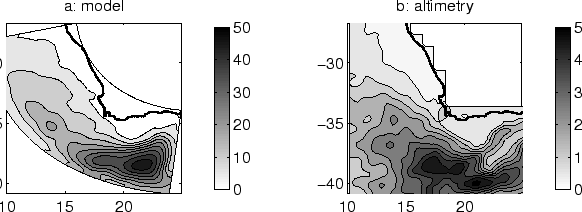 |
The root mean square of the sea surface elevation has been computed at high
resolution (0.25) from combined Topex-Poseidon and ERS1 altimetry data from
October 1992 to October 1997 [Ducet et al., 2000]. It shows a local maximum (50 cm) in the
Agulhas retroflection area and minimums over the shelves of the South and West coasts
(0-5 cm off the west coast and 5-10 cm of the Agulhas Bank, figure
3.41-b). Away from the open boundary sponge layers, this behavior is
remarkably well simulated, qualitatively and quantitatively, in the high resolution
experiment (figure 3.41-a). Difference between the model and the
altimetry variance in sea surface elevation is present around 17.5 E and 37
S, in the pathway of the Agulhas rings. At this location, a maximum in sea surface
elevation variance is noticeable in the altimetry data, but is not present in the
outputs of the model simulation. This discrepancy can be related, as explained
previously, to the vicinity of the open boundary not allowing the Agulhas
rings
to evolve properly.
Figure 3.42:
Subsurface (-50 m depth) eddy kinetic energy (cm.s). a: from
the high resolution experiment. b: from satellite altimer data. The interval
between the isocontours is 100 cm.s. The horizontal coordinates account
for the longitude and the latitude.
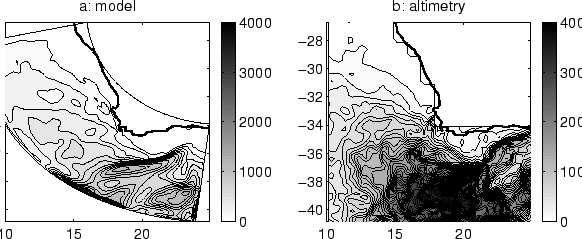 |
The eddy kinetic energy per unit of mass
 has
been also derived from high resolution altimetry data [Ducet et al., 2000]. It also shows
an important maximum in the Agulhas retroflection area (4000 cm.s). The
variations in the incoming Agulhas Current correspond to a narrow band of high
eddy kinetic energy ( 2000 cm.s) (figure 3.42-b). North of
35 S and West of 20 E, the subsurface eddy kinetic energy (computed for z =
-50 m) coincides qualitatively and quantitatively with the observed eddy kinetic
energy (figure 3.42-a). This shows that the eddies formed from the Cape
Peninsula and Cape Columbine have a correct behavior. Because the incoming Agulhas
Current is forced at the eastern boundary from smooth climatology data the remote
variations in the Agulhas Current, like Natal pulses and meanders, are not resolved
by the model. Hence, very low eddy kinetic energy is present along the eastern part
of the Agulhas Bank in comparison to the observations. As a consequence, the
simulated eddy kinetic energy is 2 times smaller than the observations in the
retroflection area.
has
been also derived from high resolution altimetry data [Ducet et al., 2000]. It also shows
an important maximum in the Agulhas retroflection area (4000 cm.s). The
variations in the incoming Agulhas Current correspond to a narrow band of high
eddy kinetic energy ( 2000 cm.s) (figure 3.42-b). North of
35 S and West of 20 E, the subsurface eddy kinetic energy (computed for z =
-50 m) coincides qualitatively and quantitatively with the observed eddy kinetic
energy (figure 3.42-a). This shows that the eddies formed from the Cape
Peninsula and Cape Columbine have a correct behavior. Because the incoming Agulhas
Current is forced at the eastern boundary from smooth climatology data the remote
variations in the Agulhas Current, like Natal pulses and meanders, are not resolved
by the model. Hence, very low eddy kinetic energy is present along the eastern part
of the Agulhas Bank in comparison to the observations. As a consequence, the
simulated eddy kinetic energy is 2 times smaller than the observations in the
retroflection area.
Figure 3.43:
Top:
subsurface (-50 m depth) velocity-variance ellipses. One ellipse is portrayed every
6 grid points. Bottom: velocity-variance ellipses from the times series components
derived from Geosat altimetry data, adapted from Morrow et al. [1994]. The scale is
the same in each portrayal, represented by the ellipse in the bottom-left corner of
the top panel.
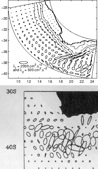 |
The eddy kinetic energy shows that important variability occurs near steep
topography around the South West corner of Africa. Hence, we can expect the
variability to be strongly anisotropic. This as been observed from satellite
altimer data [Morrow et al., 1994]. An analysis is conducted to see if the model reveals
this
anisotropic aspect of the current variability. The magnitude and the direction of
the eddy variability are represented as in Morrow et al. [1994], using variance
ellipses. The current variations being  and
and  , following Morrow et al.
[1994], the direction of the major axis of variability, measured anti-clockwise
from the direction of the u velocity component is:
, following Morrow et al.
[1994], the direction of the major axis of variability, measured anti-clockwise
from the direction of the u velocity component is:
 |
(106) |
where  is the variance along the major axis and is given by
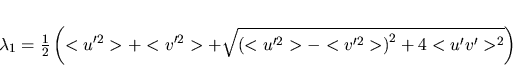 |
(107) |
and  is the variance along the minor axis given by
 |
(108) |
Note that the eddy kinetic energy ( ) is connected to the velocity
variance by
) is connected to the velocity
variance by
 |
(109) |
The subsurface variances ellipses are represented for the high resolution
model for z = -50 m (figure 3.43-top). They show a high degree of
similitude with the variances ellipses derived from Geosat satellite altimer data
(figure 3.43-bottom). The remarks made for the eddy kinetic energy
are also valid for the variances ellipses: good comparison along the west coast, whilst
the ellipses are smaller for the model outputs in the Agulhas retroflection
area. The incoming variability pattern of the Agulhas Current is illustrated by the
two elongated ellipses on the Eastern part of the Agulhas Bank for the satellite
analysis (figure 3.43-bottom). This shows important cross isobath
variations (characteristic of the meanders and natal pulses) in the Agulhas Current
around 23 E. As explained previously, this variability generated upstream of
the area is not resolved by the model. As a consequence, the simulated variability
in the Agulhas retroflection area is two times smaller than the observations. Both
the model results and the observations show an important anisotropy in the
variability, mostly near strong topographic gradients. This anisotropy is
important along the southern tip of the Agulhas Bank. The variability appears to be
more isotropic on the south west of the Agulhas Bank (where the Agulhas rings are
shed) for the observations. This behavior is not noticeable in the model
solution, the Agulhas rings being quasi-immediately in contact with the offshore open
boundary. Along the West Coast, where altimeter data are available, the model and
satellite variances ellipses compare fairly well. This is especially true near the Cape
Peninsula, where the presence of the cape induces a strong anisotropy in the
subsurface current variability. Animations of the model output reveals that
cyclonic eddies are mostly generated from Cape Columbine, Cape Peninsula and the
Southern tip of the Agulhas Bank. These areas of eddy generation coincides with
areas of strong anisotropy of the current variability. Another interesting feature
is the anisotropy of the variability close to the open boundaries. It happens that
the open boundary inhibits the cross boundary velocity variance. This can be an
effect of the Flather open boundary scheme that constrains the cross boundary
barotropic velocities to remain close to smooth climatology data values.
One can conclude from this section that though the strong variations in the
Agulhas Current coming from the Indian Ocean are not taken into account in
the model solution, and disregarding the Agulhas ring behavior when they have a size
comparable to the model width, the variability developed in the model in the form of
eddies, plumes,... compares remarkably well to observations. This is particularly
true along the South African West Coast.
4 Along the West Coast
Because of its importance for the biological components, the model solution of the
Benguela upwelling system along the South African West Coast is analyzed in more
detail.
Figure 3.44:
sea
surface temperature along the west coast of South Africa the 30 November of model
year 4.
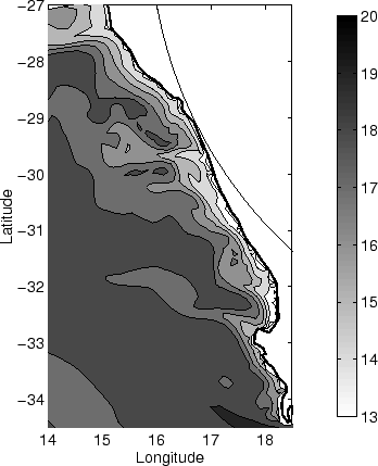 |
The upwelling system is characterised by the presence of cold water at the coast
induced by the Ekman divergence forced by the summer equatorward winds. As
explained
in the first chapter, the resulting upwelling front is highly convoluted and shows
characteristic patterns such as the upwelling plumes extending from Cape Peninsula,
from Cape Columbine and from the Namaqualand upwelling centers around 30.5 S.
Other characteristic features are the cyclonic eddies that are shed from the capes.
Because these patterns have been mostly related to the small scale spatial and
temporal structure of the wind forcing
[Jury, 1985a,Jury, 1985b,Jury et al., 1985,Jury, 1986,Jury and Taunton-Clark, 1986,Jury, 1988,Kamstra, 1985,Taunton-Clark, 1985], one might expect that a
model solution only forced by a coarse smooth climatological wind field (see figure
3.10) should not generate these elements, characteristic of the Benguela
upwelling system. This is not the case. Looking at the modelized sea surface
temperature at the beginning of the upwelling season, the 30 November of model year
4
(figure 3.44), one can note that most of observed patterns of the
upwelling front are present during the high resolution experiment:
- A small cyclonic eddy, characterized by core of colder water located at
17.2 E and 33.6 S, has detached from the Cape Peninsula upwelling center and
is advected in a north-westward direction.
- A large upwelling plume, showing the characteristic inverted s shape described
by Shannon [1985], extends from Cape Columbine.
- Upwelling filaments extend from a well defined Namaqualand upwelling center at
30.5 S.
The shape and dimensions of these simulated features
compare well with the observations. Hence, the mesoscale activity of the Benguela
upwelling system is driven by intrinsic oceanic instability processes and is
triggered by topography, as explained by Batten [1997]. The small scale
wind structure doesn't appear to be the main driving forcing of this mesoscale
activity.
Figure 3.45:
a:
the South and West Coast time averaged currents (cm.s) at 30 m depth. One
vector is portrayed every 3 vectors. b: along shore current (cm.s, positive
towards the equator) cross section North of Cape Columbine. The greyscale range
represents the equatorward along shore current in cm.s. The isocontour
interval is 5 cm.s. The position of the cross section is given by the dashed
line on panel a
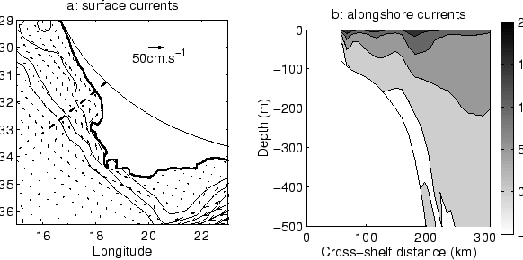 |
The time averaged subsurface modelized currents are highly controlled by the
topography (figure 3.45-a). A large amount off Acoustic Doppler
Current Profilers data has been collected by Boyd and Oberlholster [1994] to
generate
a time averaged map of the 30 m depth currents on the shelves of the South and West
coasts of South Africa. Important quantitative similitude occurs in the comparison
between the model outputs and the ADCP data:
- A reverse flow of about 10 cm.s is visible on the 200 m isobath on the
Eastern Agulhas Bank.
- A sluggish circulation is present on the Agulhas Bank.
- A shelf edge jet of about 25 cm.s flows from the Southern tip of the
Agulhas Bank towards Cape Peninsula and Cape Columbine.
- A convergent flow occurs on the western margin of the Agulhas Bank to fill the
Cape of Good Hope jet.
- The flow North of Cape Columbine follows the 200 m isobath that curves inshore
at 31.5 S and moves offshore at 30 S with characteristic velocities of 20
cm.s.
The principal discrepancy between the model and ADCP data is the current in St
Helena Bay, in a narrow band just North of Cape Columbine. For the ADCP data, the
flow in St Helena Bay is weak and show a cyclonic motion, as explained by Holden
[1985] and simulated by the barotropic experiment in the second chapter. For the
realistic simulation, an important flow of 20 cm.s, follows the Northern part
of Cape Columbine to fill St Helena Bay. The results of the second chapter might
give an explanation of this phenomenon. In the barotropic experiment, the sluggish
circulation is present inside the attached cyclonic eddy that develops on the flat
portion of the shelf where the dynamics are controlled by a balance between advection
of vorticity and bottom friction. Although weighted by
 , the
Shapiro filter employed to smooth the bottom topography for the realistic experiment
removed the flat portion of the shelf in St Helena Bay. The resulting bottom
topography corresponds more to the exponential topography employed for the
analytical standing shelf wave solution (figure 2.14). In the case of
the exponential topography, the vortex stretching term gains importance and the flow
sticks to the downwind side of the cape (figure 2.17-a) as for
the realistic experiment.
A cross-shelf cross section of the time averaged along shore velocities North of
Cape
Columbine for the upper 500 m depth is portrayed on figure
(3.45-b). It shows an equatorward baroclinic jet of 20
cm.s above the shelf break. A net poleward motion with velocities of 5
cm.s is present on the shelf break in agreement with the current meter
measurements of Nelson [1989]. A subsurface poleward current is also present at the
coast with velocities of 5 cm.s. This is also in agreement with
observations [Boyd and Oberholster, 1994,Nelson, 1989].
, the
Shapiro filter employed to smooth the bottom topography for the realistic experiment
removed the flat portion of the shelf in St Helena Bay. The resulting bottom
topography corresponds more to the exponential topography employed for the
analytical standing shelf wave solution (figure 2.14). In the case of
the exponential topography, the vortex stretching term gains importance and the flow
sticks to the downwind side of the cape (figure 2.17-a) as for
the realistic experiment.
A cross-shelf cross section of the time averaged along shore velocities North of
Cape
Columbine for the upper 500 m depth is portrayed on figure
(3.45-b). It shows an equatorward baroclinic jet of 20
cm.s above the shelf break. A net poleward motion with velocities of 5
cm.s is present on the shelf break in agreement with the current meter
measurements of Nelson [1989]. A subsurface poleward current is also present at the
coast with velocities of 5 cm.s. This is also in agreement with
observations [Boyd and Oberholster, 1994,Nelson, 1989].
Figure 3.46:
a:the
South and West Coast time averaged barotropic currents (cm.s). All velocity
vectors are represented. b: annual averaged free surface elevation. The greyscale
range represents the free surface elevation in m.
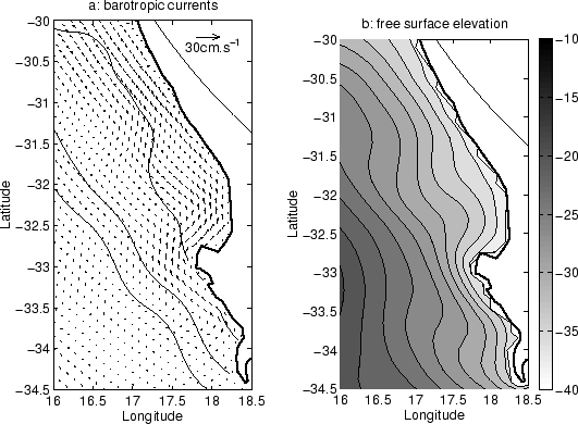 |
In order to compare the output of the realistic simulation to the results of the
second chapter, the time averaged barotropic velocities and free surface
elevation are portrayed for a small area centered on St Helena Bay in figure
(3.46). Note that in presence of a baroclinic pressure gradient
induced by the stratification, the baroclinic velocities are no longer in geostrophic
equilibrium due solely to the pressure gradient induced by free surface elevation. The
annual averaged along shore wind stress utilized to force the model in the area
limited by the bounds of figure (3.46) is 0.5 N.m. The
characteristic barotropic velocities on the shelf in figure
(3.46-a) are of about 7.5
cm.s which is slightly smaller than the values obtained in section
(2.8) for the case of the exponential shelf for this wind forcing.
For both the barotropic velocities and the free surface elevation, a standing wave
pattern is noticeable in the lee of Cape Columbine (figure
3.46-a). It has a wave length of approximately 100 km.
The wave length for the first barotropic standing wave mode derived in section
(2.8), using an exponential topography and an along shore mean
current of 7.5
cm.s is 60 km. This is 1.6 times smaller than the wave length observed in
the realistic experiment. Different arguments can be advanced to explain this
difference: firstly, one can note that the topography of the realistic experiment
is
not constant along West Coast, with the 200 m isobath moving towards the coast
around
31.5 S. This can alter the vorticity equation employed to derived the standing
wave equation. Secondly, the presence of stratification can alter the behavior of
the standing coastal trapped waves. Looking at the dispersion relation for coastal
trapped waves for different stratification [Huthnance, 1978], one can note that the
wave length decreases for a given phase velocity (hence for a fixed advection by a
mean along shore current in the standing wave case) with increasing stratification,
invalidating this second argument. Thirdly, the hypothesis made in section
(2.8) that the along shore mean current is barotropic is surely not
valid in the realistic case where the along shore currents associated with the
upwelling
are a surface baroclinic jet. The process of a standing barotropic shelf wave
excitation by a baroclinic surface jet has not been treated in section
(2.8). In this case, the model of a cape moving in still water
is invalid. Surprisingly, if we introduce the subsurface velocity observed
on figure (3.45) as the mean along shore current (20
cm.s)
in the standing wave equation, we obtain exactly 100 km for the wave length of the
first mode. This can not be taken as a proof. Nevertheless, we still can
note that the time averaged circulation simulated on the shelf in St. Helena Bay for
the realistic experiment is qualitatively in agreement with the results of the
standing shelf wave analytical study of section (2.8).
Figure 3.47:
a:
south and west coast averaged barotropic currents (cm.s) for February. All
velocity vectors are represented. b: averaged free surface elevation for February.
The greyscale range represents the free surface elevation in m.
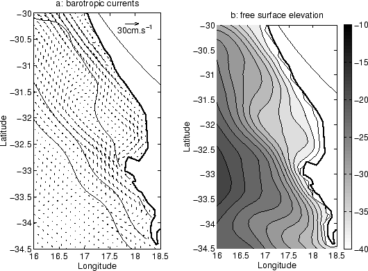 |
The same analysis is made for the middle of the upwelling season: for the month of
February (figure 3.47). For this particular month, the along
shore wind stress on the west coast has an averaged value of 0.075 N.m. The
averaged barotropic currents portrayed in figure (3.47-a) have a
characteristic velocity of about 10 cm.s. An interesting feature in
figure (3.47) is the separation of the flow into 2
branches past Cape Columbine: one branch filling St Helena Bay, the other one
flowing north westward parallel to the coastline to come back to the coast 150 km
North of Cape Columbine. This is characteristic of the Columbine divide described
by Shannon [1985] (figure 1.13). Whereas the inner branch shows a
standing wave pattern comparable of the annual averaged circulation, the behavior
of the outer branch resembles the attached cyclonic eddies modelized in the second
chapter. For this value of wind stress, the size of the eddy described in chapter 2
is 60 km (figure 2.6), which is smaller than the size of the
detachment pattern observed in figure
(3.47). On the contrary the length scale predicted by the
balance between advection and bottom friction (equation 2.21)
is 125 km, which is relatively close to the size of the pattern observed in figure
(3.47). This last result should be taken cautiously, since
stratification or variations in bottom topography can seriously alter the
circulation within St. Helena Bay.
5 Generation of cyclonic eddies by the Agulhas Current in the lee of the
Agulhas Bank
Though the realistic configurations have been principally set up to study the shelf
dynamics around the South-west corner of the African continent, and particularly the
Benguela upwelling system, the results of model regarding the
Agulhas Current has motivated the redaction of two papers. They focus attention
on specific mesoscale processes produced by the model, observed in nature, and not
simulated before in this area. The present section
describes the generation of cyclonic eddies by the Agulhas Current in the lee of the
Agulhas Bank [Penven et al., accepted]. The second paper, still in preparation, forms the next
section.
The inter-ocean exchanges brought about by the shedding of Agulhas rings south-west
of Africa has been much studied because of their global climatic implications [
Lutjeharms, 1996; De Ruijter et al., 1999]. Recent models have shown that
this movement of warm water from the Indian to the Atlantic may in fact control the
rate of thermohaline overturning of the whole Atlantic [Weijer et al., 1999]. There are also
other, smaller sources of exchange including Agulhas filaments [Lutjeharms and Cooper, 1996] and
intrusions of cold subantactic water [Shannon et al., 1989]. In addition, a number of cold,
cyclonic eddies have been observed in the South-east Atlantic [e.g.
Duncombe Rae et al., 1996; Gründlingh, 1995]. For a proper
quantification of the inter-ocean exchanges the characteristics of all these
components need to be known. The origin, behavior and potential role in
inter-ocean exchanges of the cyclonic eddies have not been established.
We verify if the high resolution model might simulate these cyclonic eddies,
and we investigate the origin of such cyclonic eddies.
Figure 3.48:
(a)
Model simulation of the sea surface height and barotropic velocities (1 vector every
4 grid points) on 27 April of model year 2. (b) Naval Research Laboratory, MODAS
2.1, sea surface height derived from in-situ and satellite altimetry data on 16
January 1993.
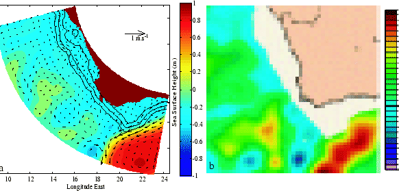 |
The model gives a realistic portrayal of the known circulation in this ocean region
(figures 3.48-a and 3.50-b), including mesoscale details such as
the Agulhas Current, shear edge features on the landward border of the current,
Agulhas rings and the wind-driven coastal upwelling along the west coast. The
Agulhas Current overshoots the concave eastern part of the Agulhas Bank and has its
maximum surface velocities of about
1 m.s at the southernmost tip of the shelf. These simulations are all in
very good agreement with observation [e.g. Lutjeharms et al., 1989]. The
features evident in the modeled sea surface height are also well represented in
the sea surface height observed by altimetry
(figures 3.48-a and 3.48-b). These consist of an anti-cyclonic
Agulhas ring as well as some cyclonic eddies of unknown origin. One of these
cyclonic eddies lies between the Agulhas Current and the western side of the Agulhas
Bank in both portrayals. Cyclonic eddies are prevalent at this particular location
in the model and this portrayal is therefore quite characteristic in this respect.
Figure 3.49:
The
drift patterns for a few characteristic cyclonic eddies west of the continental
shelf. The bold tracks are for model eddies shed during model year 3; the dotted
tracks for cyclones observed in Naval Research Laboratory, MODAS 2.1 sea surface
height analysis for 1993.
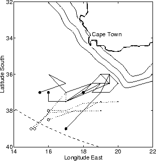 |
An analysis of the generation, drift and persistence of cyclonic eddies at this
location as observed in satellite altimetry is highly consistent with the model
simulations (figure 3.49). They are formed at roughly the same location,
drift off in the same westerly direction, are produced with the same frequency, and
can dissipate rapidly or grow in intensity. These results give us confidence that
these features are not model artifacts. It would be important to establish the
depth and other hydrographic characteristics of these particular cyclonic eddies.
Figure 3.50:
A
comparison between a characteristic cyclonic eddy generated off the Agulhas Bank in
the model (b and d) and one observed at sea (a and c). The panel b shows the
simulated surface currents and sea surface temperature on 21 November of model year
4. It also shows the line along which a vertical temperature section (d) has been
extracted from the model at the same date. The sea surface temperature generated
from NOAA 11 AVHRR data (a) is for 27 November 1992. The straight broken line shows
the cruise track of the research vessel "Polarstern" that left Cape Town on 3
December 1992. The dotted line shows the location of the warm filament on 4
December 1992 when the vessel would have been in the center of this feature. The
vertical temperature section (c) was measured by XBT (expendable bathythermograph)
from the ship. The locations of the 200 m, 500 m and the 1000 m isobaths are shown
in panels a and b.
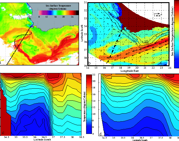 |
The sea surface temperature and current portrayals in the upper panels of figure
(3.50) exhibits substantial agreement. The model shows a plume of warm
surface water that encircles a cyclonic eddy in the lee of the continental shelf
(figure 3.50-b). To the North, there is faint indication of an
anti-cyclonic
eddy in the current vectors, encircled by the extension of the warm filament. The
satellite thermal infrared image shows much the same (figure 3.50-a),
except that the locations of the two features are slightly displaced. A vertical
temperature section through the two eddies in the model shows the warm surface
filaments as well as an anti-cyclonic eddy centered at 35.3 S and a cyclonic
eddy at 36.7 S (figure 3.50-d). In the model, the eddy is
still noticeable at 1500 m depth. An XBT
section was undertaken across this region in a very similar location [Bathmann et al., 1994].
It is shown in the left-hand panels of figure (3.50). Regrettably, the
sea surface temperature image was largely obscured by cloud on the day of the
hydrographic section. Nonetheless, the position of the feature could be located and
is shown relative to that of the 27 November 1992 by the dotted line in figure
(3.50-a). The vertical temperature section for this line resembles
closely that of the model, both in the surface filaments as well as in the presence
of both a cyclonic as well as an anti-cyclonic eddy (figures 3.50-c and
3.50-d). The strong resemblance of the hydrographic and model results
shows that the cyclonic eddies generated off the Agulhas Bank in the model are not
inconsistent with observations and extend to substantial depths.
In the model, the coastal part of the Agulhas Current tends to follow the
topography at the southern tip of the Agulhas Bank, carrying warm
surface filaments spreading northward towards Cape Peninsula. At
times, the southern part of this flow detaches from the topography and
a cyclonic meander developes. After approximately 1 month, it detaches
from the Agulhas Bank, taking away the warm filament (see Figures 3-a
and 3-b). Occasionally, a cyclonic perturbation may follow the shelf
break from the eastern Agulhas Bank and trigger the cyclonic eddy
generation process. The averaged values of the Rossby ( ) and
Burger (
) and
Burger ( ) numbers have been computed as described in
Boyer and Tao [1987], taking the width of the Agulhas
Current as a characteristic length scale (100 km). They lie in the
cyclonic eddy shedding regime found in rotating tank experiments, when
a linearly stratified flow encounters an obstacle [Boyer and Tao, 1987]. Thus,
the generation of cyclones past the Agulhas Bank can be explained
by a flow detachment process. Their characteristic diameters range
from 50 km to 200 km. Although they are generated irregularely, the
number of eddy shed each year is relatively constant, respectively
from year 1 to year 10: {3,3,4,4,4,5,4,5,4,5}. Because the model
domain has a limited size, most of the cyclonic eddies are radiated
through the offshore boundary before decaying (figure 3.49).
The first simulations of the southern Agulhas Current by a model with high spatial
resolution suggests that the disposition of the current relative to the southernmost
part of the African continental shelf is such that cyclonic lee eddies may be
generated. This may be an intermittent process since the Agulhas Current does not
follow the most southerly part of the shelf consistently [Lutjeharms et al., 1989]. The model
indicates that these eddies may be shed at irregular intervals. They may
subsequently move off in a number of directions in the South-West Indian Ocean
[Gründlingh, 1995]. Their further dispositions, their contribution to the melange of
water masses in this ocean region as well as their potential role in stabilizing
Agulhas rings (Kizner, personal communication) all need to be determined. If all
cyclonic rings in the south-western Atlantic have this suggested origin, they will
not contribute to inter-ocean exchanges since they are generated in situ.
) numbers have been computed as described in
Boyer and Tao [1987], taking the width of the Agulhas
Current as a characteristic length scale (100 km). They lie in the
cyclonic eddy shedding regime found in rotating tank experiments, when
a linearly stratified flow encounters an obstacle [Boyer and Tao, 1987]. Thus,
the generation of cyclones past the Agulhas Bank can be explained
by a flow detachment process. Their characteristic diameters range
from 50 km to 200 km. Although they are generated irregularely, the
number of eddy shed each year is relatively constant, respectively
from year 1 to year 10: {3,3,4,4,4,5,4,5,4,5}. Because the model
domain has a limited size, most of the cyclonic eddies are radiated
through the offshore boundary before decaying (figure 3.49).
The first simulations of the southern Agulhas Current by a model with high spatial
resolution suggests that the disposition of the current relative to the southernmost
part of the African continental shelf is such that cyclonic lee eddies may be
generated. This may be an intermittent process since the Agulhas Current does not
follow the most southerly part of the shelf consistently [Lutjeharms et al., 1989]. The model
indicates that these eddies may be shed at irregular intervals. They may
subsequently move off in a number of directions in the South-West Indian Ocean
[Gründlingh, 1995]. Their further dispositions, their contribution to the melange of
water masses in this ocean region as well as their potential role in stabilizing
Agulhas rings (Kizner, personal communication) all need to be determined. If all
cyclonic rings in the south-western Atlantic have this suggested origin, they will
not contribute to inter-ocean exchanges since they are generated in situ.
6 Shear edge eddies of the southern Agulhas Current
The southern and the northern parts of the Agulhas Current consistently exhibit
differences in their path characteristics. Whereas the trajectory of the northern
part is unusually stable for a western boundary current [Gründlingh, 1983], the southern
part has large meanders [Harris et al., 1978,Lutjeharms, 1981]. This contrasting kinematic behavior is
a consequence of the steepness of the continental shelf slope [De Ruijter et al., 1999a]. A very
steep slope and narrow continental slope constrains the northern part of the current
whereas a more gradual slope along the wider continental shelf south of Africa (the
Agulhas Bank) allows more side-ways meandering. The exception is a small region of
weaker slope along the northern Agulhas Current, at the Natal Bight, where small
meanders and accompanying eddies have also been observed [Gründlingh and Pearce, 1990] along the edge
of the current. Cyclonic eddies are embedded in the landward border of current
meanders in the southern Agulhas Current and seem to gain energy from the lateral
shear due to the juxtaposition of fast moving water in the current and more sluggish
water over the shelf. These cyclonic shear eddies may have a substantial influence
on adjacent shelf waters of the Agulhas Bank. They are usually attended by warm
plumes drawn from the surface waters of the current
[Harris et al., 1978,Lutjeharms, 1981,Schumann and van Heerden, 1988,Lutjeharms et al., 1989,Goschen and Schumann, 1990]. These plumes have in fact been the prime
manifestation of shear edge eddies that has been used for their study by thermal
infrared sensing from satellite. Depending on the reigning wind conditions, this
anomalously warm surface water may then spread over substantial parts of the
adjacent shelf [Lutjeharms et al., 1989,Goschen and Schumann, 1994]. It has even been surmised [Swart and Largier, 1987] that this
warm surface water may thus make an important contribution to the intense seasonal
thermocline over the eastern part of the Agulhas Bank [Schumann and Beekman, 1984]. This
hypothesized contribution has as yet not been quantified. Regrettably, few of these
shear edge eddies have to date been hydrographically surveyed. A study by
Lutjeharms et al. [1989] has used two sets of hydrographic observations as well as
satellite imagery to give a general description of these features. More eddies are
found the further downstream one measures. In general their lateral dimensions also
increase downstream. They seem to be particularly prevalent in the shelf bight on
the eastern side of the Agulhas Bank. Judged by the trailing plumes of warm water,
they all move downstream, but an insufficient number of time series in the satellite
imagery has prevented a statistically reliable propagation speed to be derived.
Once past the southern tip of the Agulhas Bank, warm plumes may be advected
equatorward into the southern Atlantic Ocean, making a modest contribution to the
inter-ocean leakage of heat and salt [Lutjeharms and Cooper, 1996]. The fate of the eddies
themselves remains unknown. Shear edge eddies my have a diameter of about 50-100 km
and are represented by a well-defined thermal dome (figure 3.53-b)
inshore of the landward border of the Agulhas Current. This portrayal of these
eddies is complicated by the intermittent passage of a Natal Pulse through the
region. Natal Pulses are substantial, single meanders in the trajectory of the
Agulhas Current [Lutjeharms and Roberts, 1988] that are generated by current instability at the Natal
Bight [De Ruijter et al., 1999a] and that propagate downstream at a rate of about 20 to 30
km.day. When they move past the Agulhas Bank, they seem to slow down to
roughly 5 km.day [Lutjeharms and Roberts, 1988,Van Leeuwen et al., 2000] and become difficult to distinguish from
the other meanders normally found here. Like these other meanders, Natal Pulses
also incorporate cyclonic eddies [Gründlingh, 1979] that move downstream with them. Once
past the southernmost tip of the Agulhas Bank, Natal Pulses may trigger the shedding
of an Agulhas ring [Van Leeuwen et al., 2000] by loop occlusion at the Agulhas retroflection
[Lutjeharms and van Ballegooyen, 1988]. The role this process plays in interocean exchanges South of Africa
has been extensively reviewed by De Ruijter et al. [1999b] and Lutjeharms [1996].
It is not known what happens to the cyclone that is carried in a Natal Pulse once
the meander has passed the tip of the Agulhas Bank. There is evidence that a
cyclonic eddy may on occasion be generated in the lee (western side) of the Agulhas
Bank by the passing Agulhas Current [Penven et al., accepted] and it has been surmised that the
cyclonic eddy that comes with a Natal Pulse may be absorbed by such a lee eddy.
Similarly, it has been hypothesized that shear edge eddies may be absorbed by
cyclonic eddies in a passing Natal Pulse, thus enhancing it and even contributing to
the efficaciousness with which it influences Agulhas ring shedding downstream.
The outputs of the high resolution experiment are employed in order to understand
the
processes involved in the generation and subsequent behavior of shear edge eddies
Figure 3.51:
Sea surface temperature (C) and surface currents (m.s) over the
Agulhas Bank for the 10 April of model year 9. The greyscale range represents the
sea surface temperature in C. The interval between the isocontours is 0.5
C.
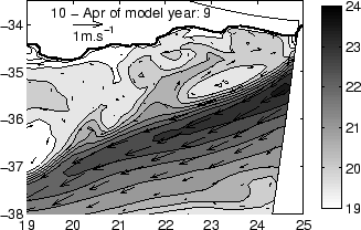 |
The sea surface temperature over the Agulhas Bank for the 10 April of model year 9
is given in figure (3.51). Simulated surface currents are also
shown. Temperatures in the core of the Agulhas Current are 23C and 24 C and
decrease downstream. Temperatures on the shelf lie between 18 C and 20C .
These values are all very representative for these features for this time of year
[Schumann and Beekman, 1984,Lutjeharms, 1996]. The core of the Agulhas Current does not follow the shelf edge
very rigorously, but overshoots the bight in the Agulhas Bank at about 23 E, and
eventually crosses the 1000 m isobath at the southernmost tip of the shelf (figure
3.51). Velocities in the current are up to 1 m.s; over the
Agulhas Bank in general much lower ( 20 cm.s). Both these values are very
realistic [Schumann and Perrins, 1982]. Two surface plumes of warm water at the inshore edge of the
Agulhas Current are evident in figure (3.51). A small plume lies
at 2030' E, the larger one starts at 22 E. The latter represents a fully
developed shear edge feature around the concave part of the shelf break with surface
counter currents of up to 40 cm.s. The implied shear edge eddy has
dimensions of approximately 80 by 150 km. These simulations of the surface
characteristics of this region show a high verisimilitude to those evident in figure
(3.53-a) and give a most realistic portrayal of the known conditions
for the region, i.e. for this time of the year.
Figure 3.52:
The
simulated sea surface temperature (C) for the Agulhas Bank and direct vicinity
for a: 2 June, b: 2 August, c: 2 October and d: 2 December of model year 7. The
greyscale range represents the sea surface temperature in C. The interval
between the isocontours is 1 C. The dashed lines represent the 200 m, 500 m and
1000 m isobaths.
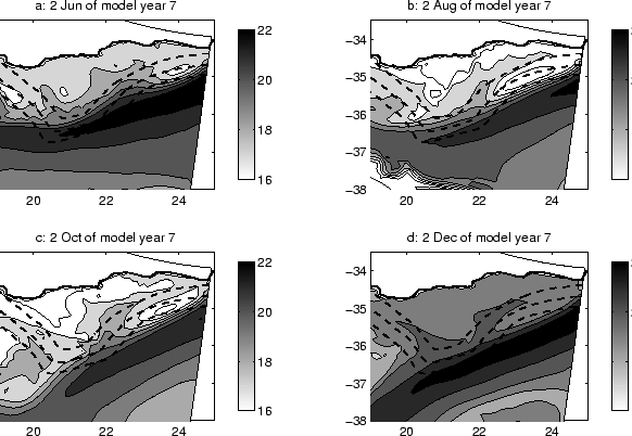 |
A portrayal of model results for all seasons of model year 7 is given in figure
(3.52). Two aspects of the inter-seasonal variability for the sea
surface is immediately apparent. The first is the expected seasonal temperature
variations. Both the temperatures in the core of the Agulhas Current and those of
the shelf waters exhibit a seasonal cycle of at least 2C. These values also are
realistic [Christensen, 1980]. The second thing that is clear is that the location of the
simulated Agulhas Current is not entirely stable. This is particularly noticeable
downstream of the Agulhas Bank - from June to October the current shifted by at
least 240 km. Along the eastern edge of the Agulhas Bank, the meandering of the
Agulhas Current is less noticeable, but inspection of its location at about 23 E
in June (figure 3.52-a) and in October (figure 3.52-c)
shows a noticeable southward shift. The main shear edge eddy is a recurrent feature
of the Agulhas Bank bight, but may lie farther upstream (figure 3.52-a)
or downstream (figure 3.52-d). Figures (3.51) and
(3.52) therefore demonstrate that the model simulates the known surface
conditions very well.
Figure 3.53:
a:
distribution of temperature (C) at 10 m over the Agulhas Bank in March 1968. b:
Temperature cross section across a border eddy south of Mossel Bay. Adapted from
Lutjeharms et al. [1989].
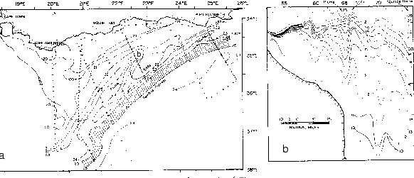 |
Figure 3.54:
a: This panel is identical to that in Figure (3.51). The
broken line indicates the location of a simulated vertical section from the land
across the shelf and shelf edge an crossing the edge of the Agulhas Current that is
given in the right panel. b: A vertical temperature section to 200 m depth along
the broken line in the upper panel. Note the warm water of the Agulhas Current, the
dome of cold water forming a shear eddy and the plume of warm water extending to a
depth of 20 m.
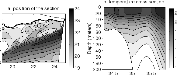 |
Figure 3.55:
a:
distribution of temperature (C) at 10 m over the Agulhas Bank in September 1968.
b: Temperature cross section across a border eddy south of Mossel Bay. Adapted
from Lutjeharms et al. [1989].
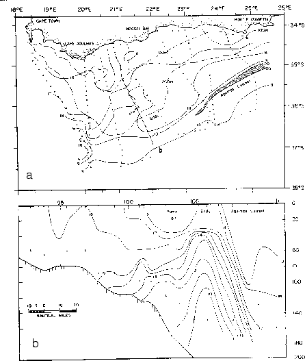 |
Figure 3.56:
a:The sea surface temperature (C) simulated for 15 September of model
year 7. Otherwise as in Figure (3.51). The broken line indicates
the location of a simulated vertical section from the land across the shelf and
shelf edge an crossing the edge of the Agulhas Current that is given in the right
pane. b: potential temperature (C) vertical section to 200 m along the line.
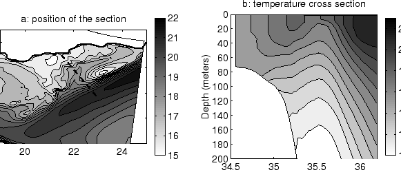 |
To judge the full effectiveness of the model, one would want to test this in the
vertical as well. A vertical section is shown in figure (3.54).
The simulated section in this figure is taken across the eastern Agulhas Bank,
across a warm plume, a shear edge eddy as well as the landward edge of the Agulhas
Current. The location as well as the time of year has been selected to make
comparison easier with a hydrographic section taken at this location and portrayed
in figure (3.53-b). The main features are represented well,
including the thermal gradient of the edge of the Agulhas Current, the shape and
size of the cold dome representing the eddy as well as the depth and shape of the
warm surface plume heading upstream. The plume overlies the landward edge of the
eddy, as represented by the strongest horizontal, sub-surface temperature gradient.
This corresponds to what has been observed in nature [Lutjeharms et al., 1989]. Even the
vertical gradient of the seasonal thermocline over the Agulhas Bank is entirely
representative for this time of year [Lutjeharms et al., 1996]. Shear edge eddies are also
present in winter as can be seen in figure (3.56) for the model
and in figure (3.55) for hydrographic data. For this time of the
year, the thermic vertical structure is also remarkably well represented by the
model, showing a relatively homogeneous temperature (15C) onto the Agulhas Bank
(figures 3.56-b and 3.55-b). The sea surface
temperature shows the warm plume that rounds the shear edge eddy both in the model
(figure 3.56-a) and in the hydrographic data (figure
3.56-a). The reverse plume appears to be further downstream
( 100 km) in the hydrographic data than in the model results. At this time of
the year, the cold dome happens to be more marked than in summer. Regrettably there
are insufficient data on shear edge features of the Agulhas Current to afford more
inter-comparisons between the model simulations and actual observations.
Nonetheless, those that have been presented here are such that they give us
considerable confidence in the reliability of the model.
Figure 3.57:
The simulated evolution of shear edge eddies along the eastern side of the
Agulhas Bank. The broken lines denote the 200 m, 500 m and 1000 m isobaths. Shown
is the sea surface height (contour lines from -60 to 20 cm, the latter being the
value south of the Agulhas Current). The interval between the isocontours is 5 cm.
The dates are a: 7 December of model year 7, b: 15 December 7, c: 23 December 7,
d: 1 January 8, e: 7 January 8, f: 15 January 8, g: 23 January 8 and h: 1
February 8.
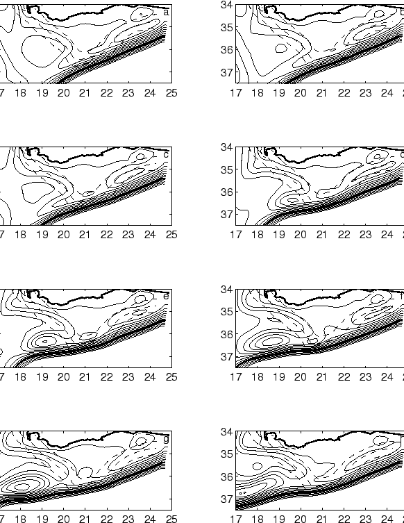 |
A time series for sea surface elevation off the Agulhas Bank and general vicinity is
portrayed in figure (3.57). It is given with 8 day intervals,
starting on 7 December of model year 7. In the first image (figure
3.57-a) there is a well-developed Agulhas Current with a large
cyclonic shear eddy in the eastern bight of the edge of the Agulhas Bank. West of
the Agulhas Bank there is a weakly developed anti- cyclone about 250 km in diameter.
The presence of an anti-cyclone in this region has been shown to occur at least 12
% of the time [Lutjeharms and Valentine, 1988]. The model also shows a small anti-cyclone in the
north-easterly corner of the modeled field over the Agulhas Bank. It remains
largely unchanged throughout the sequence. We are unsure if it is an artifact of
the boundary conditions. A week later (figure 3.57-b), the shear
edge eddy has shrunk somewhat in size, having split off a very small eddy that is
now moving downstream at about the rate such eddies are known to propagate
[Lutjeharms et al., 1989]. The anti-cyclonic eddy had grown somewhat in strength. On the next
panel these developments continue (figure 3.57-c). By 1 January
(figure 3.57-d) the smaller shear edge eddy has grown in size and
has left the eastern shelf edge. The large shear eddy in the bight has again
spawned a protrusion, this time considerably bigger. A week later this protrusion
has split of as a slightly larger eddy and is moving downstream as did its
predecessor. Its predecessor has by now developed into a strong Agulhas Bank lee
eddy, characterized by a sea surface height 25 cm lower than its South Atlantic
environment. Two weeks later (figure 3.57-g) the second shear edge
eddy had been absorbed into this lee eddy, had strengthened it to a 30 cm anomaly,
and the lee eddy can be seen moving away into the South Atlantic Ocean
[Penven et al., accepted]. Such cyclones have been observed in this region in altimetry
[Gründlingh, 1995] and from hydrographical measurements [C. Veth, S. Drijfhout,
personal communication]. They have on occasion been traced in altimetry to this
location that is associated with a lee eddy. On the last panel of this sequence
(figure 3.57-h) the lee eddy has moved totally eastward and the main
shear edge eddy is producing another downstream protrusion. Note that the
downstream leakage from this main shear eddy is always associated with a slight
offshore meander in the Agulhas Current trajectory.
Figure 3.58:
Tracking the westward leakage of cyclonic vorticity in the form of a
bud-off eddy. The left panel (a) depicts the sea surface height (5 cm between the
isocontours). Note the cores of the shear edge eddy between 23E and 24E and the
Agulhas Bank lee eddy between 18E and 19E. The broken line is used to track the
movement of water with a cyclonic motion (low sea surface height). The
Hovmüller diagram on right panel (b) shows the movement in time (increasing
upward on the ordinate). The distance on the abscissa is from the easternmost point
on the solid line in the upper panel, i.e. x=0 is at 24.25 E and 35 S; the
distances on the abscissa are positive traveling westward. The interval between
the isocontours is 3 cm.
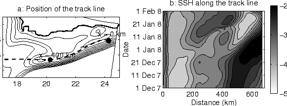 |
These images are a piecemeal selection from a more detailed series. This process
can therefore be shown with considerably better temporal resolution (figure
3.58). The left panel shows the setting for this region with the
thick broken line indicating the path along which the sea surface elevation will be
followed (figure 3.58-a). In figure(3.58-b), clear
greyscale shows low sea surface deepening in comparison to the surroundings, thus
cyclonic motion. Hence, the displacement of cyclonic shear edge eddy and the lee
eddy can be followed along the broken line by looking at low sea surface height
values. The Hovmüller diagram in the right panel (figure 3.58-b)
shows the development over time, starting at the bottom and moving upward. Note
that the direction is not the same as in the left panel (figure
3.58-a), but has been inverted. Starting from 1 December of model
year 7 (see figure 3.57-a) there is a well-developed shear edge eddy
at 100 km and an anticyclone at 500 km, i.e. in the lee of the Agulhas Bank. The
subsequent leakage of cyclonic eddies from the shear edge eddy to the lee of the
bank is shown most clearly by the clear track from the left-hand side of the panel
to the right-hand side starting on 1 January and ending at 450 km distance on 20
January. On the first
part of its trip, the shear edge eddy travels along the line at approximately 6
km.day. On the 15 January, at the Southern tip of the Agulhas Bank (x = 350
km), it accelerates up to 32 km.day. On the 20 January, it is absorbed into by
a larger cyclonic eddy developing in the lee of the Agulhas Bank [Penven et al., accepted] The
replacement of an anti-cyclone by a cyclone in the lee of the Agulhas Bank is
represented by the change from dark to clear at 500 km distance along the line on
about 1 January of model year 8. These simulations leave one with the impression
that it is the Agulhas Current that sequesters the shear edge eddy in the eastern
bight of the Agulhas Bank and, when it meanders, allows a certain part of the eddy
to escape. The cyclonic vorticity of this propagating eddy may then be taken up by
a lee eddy. How does this scenario compare to what has been observed at sea?
Satellite imagery for the region shows that warm plumes, assumed to be associated
with shear edge eddies, consistently exhibit a downstream motion. A plume might of
course be associated either with an independent, separated eddy or with the leading
edge of a protrusion from a shear eddy trapped in the eastern bight. Therefore both
possibilities remain open: there may be distinct eddies moving downstream, or
occasional protrusions still attached to a trapped eddy. Statistically, the bight
is known for the prevalence of shear edge eddies [Lutjeharms et al., 1989] so that the concept of
a near-stationary, but leaky, eddy at this location is not inconsistent with the
data. However, with very limited data it cannot be confirmed in a rigorous manner
at present. If this single simulation of the evolution of shear edge eddies at the
Agulhas Current edge seems reasonably sound, how representative is it of other such
sequences in the model?
Figure 3.59:
Hovmüller diagrams of simulations of the temporal behavior of
circulatory features along the Agulhas Bank. The sea surface elevation along the
line defined on Figure (3.58-a). The interval between the isocontours
is 3 cm. The left panel (a) represents model years 3 to 4, the central panel (b)
years 5 to 6 and the right hand panel (c) years 7 to 8. Otherwise the images are
identical to that of the lower panel of Figure 7.
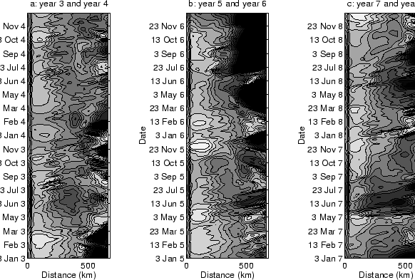 |
The simulated behavior of shear edge eddies along the edge of the Agulhas Bank for
a 6-year period in the model run is presented in figure (3.59).
Except for the extended periods the portrayal is identical to that of figure
(3.58-b). The sea surface height is tracked along the line used in
figure (3.58-b). A number of notable features are immediately
apparent. First, their is considerable inter-annual and intra-annual variation,
generated by the internal physics of the model itself. In this depiction, the
center
of the trapped shear eddy is located at a distance of 100 km in figure
(3.59). This location seems to be relatively invariant, but the
dimensions and intensity of the eddy varies considerably with time. There are
events lasting about 6 weeks when it is particularly well-developed (e.g.
November year January year 6, figure 3.59-b), and longer
periods when is seems very weak or totally absent. The absence of a trapped shear
eddy seems to coincide roughly with the presence of the Agulhas Current closer
inshore. This movement of the current is reflected by the appearance of sea surface
height elevations at a distance of about 300 km along the track and a simultaneous
sea level enhancement in the far eastern part of the domain (left side of columns in
Figure 8). On June of model year 7 (figure 3.59-c) these two
regions of higher sea level nearly touched, showing strong perturbations in the
large scale currents. At the westernmost part of the field (right side of columns
in figure 3.59) marked positive and negative departures from the
mean sea surface height show the spasmodic exchange of a cyclonic and an
anticyclonic motion. This may be interpreted as the replacement of a northward
meander in the simulated Agulhas Current with a cyclonic lee eddy (e.g. May year 3,
figure
3.59-a). Perhaps of most interest is the clear signs of
intermittent but frequent leakage of cyclonic motion (figure
3.59-b) from the upstream region to the downstream region. These
are shown as feint clear lines from left to right in the columns of figure
3.59. More marked eddy leakage can be observed on Mars 3, September
3, June 4, September 5, December 5, September 6, May 7, December 7, September 8
(figure 3.59). They indicate that these eddies that carry cyclonic
motion downstream propagate at roughly 8 km.day, very close to estimates made from
satellite imagery [Harris et al., 1978,Lutjeharms et al., 1989] for shear edge eddy progression and even for
the movement of Natal Pulses along the Agulhas Bank [Lutjeharms and Roberts, 1988,Van Leeuwen et al., 2000]. The
frequency with which there is a movement of from the trapped shear eddy downstream
seems to have some regularity if not affected by the large scale movement of the
Agulhas Current (e.g. March to November of year 4; figure 3.59-a).
The spawning of a traveling eddy seems to occur at intervals of roughly 20 days in
the model. Observations to date are insufficient to validate this, mostly due to
interference to the satellite thermal infrared measurements by cloud cover.
However, indications are of a considerably more irregular process.
The strong indication by the model that a shear eddy will get trapped in the bight
of the shelf and that this is largely determined by the interaction of the Agulhas
Current with the topography of the bight is tested in this section by a set
of idealized numerical experiments. The bight that lies at the eastern side of the
Agulhas Bank around 23 E, is characterized by the bend toward shore of the 500
m isobath, the isobaths deeper than 1500 m running quasi rectilinearly
South-westward. This creates an embayment of about 200 km long and 100 km wide. The
goal of this section is to show that the interaction between a density driven current
with a topographic accident such as the Agulhas Bight is able to generate a standing
recirculation process identical to the large shear edge eddy observed in the
realistic experiments.
Figure 3.60:
a:
bathymetry (m) employed for an idealized model of the circulation along an
indentation in a shelf slope. b: The vertical potential temperature (C)
distribution used for initial and boundary conditions, on a section from the coast
to the deep ocean.
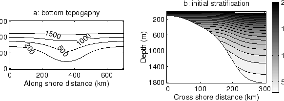 |
The ROMS model has been configured as follows:
- The grid is regular and isotropic (
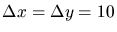 km). The length
of the domain is 700 km in the x direction and the width is 300 km in the y
direction.
km). The length
of the domain is 700 km in the x direction and the width is 300 km in the y
direction.
- For the sake of simplicity, the model domain consists of a periodic channel
along the x direction.
- The bottom topography is defined analytically and is periodic to satisfy mass
conservation in the periodic channel. Figure (3.60-a) represents the
bottom topography employed. It consists of a large shelf ending on a slope. A
perturbation of the slope in the middle of the domain account for the Agulhas Bight.
- In the vertical, 20 s-levels are evenly distributed.
- The equation of state takes a linear form depending solely on
temperature:
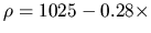 T.
T.
- All the surface fluxes are set to zero (no wind stress, no heat flux)
- No bottom flux for temperature and linear parameterization for the bottom
momentum flux:
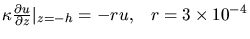 m.s.
m.s.
- The vertical mixing coefficient for momentum and temperature are constant:
 m.s,
m.s,
 m.s.
m.s.
- Figure (3.60-b) shows the cross section of the analytical
function employed for the temperature initial condition. It reproduces a typical
cross section across the Agulhas Current. The velocity and free surface elevation
are set to zero at the model start.
- The temperature is relaxed towards its initial value with a nudging time of 5
days during all the simulation.
- The Coriolis parameter f is constant equal
 . The
. The  related
processes are not taken into account.
related
processes are not taken into account.
Figure 3.61:
Sea
surface height (5 cm interval) after 60 model days. The currents have been adjusted
with the density structure. In the upper panel (a) advective terms and bottom
friction have been retained, in b there is no advection of momentum and in c both
the advection of momentum and the bottom friction have been left out.
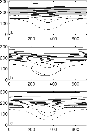 |
After 60 days of simulation, the model has reached a steady state where the
along shore velocities have been adjusted to the stratification. The resulting
surface current attains values of 90 cm.s above the 1000 m isobath. The width
of the current ranges between 50 and 100 km. We are in the parameter range of
the Agulhas Current. The resulting free surface elevation is portrayed on figure
(3.61-a). Its slope represents the along shore geostrophic surface
currents. Although the temperature is constrained to remain close
to its initial value, the free surface elevation reveals that a cyclonic
recirculation stands in the bight. Hence, this simulation shows that the interaction
between the Agulhas Current and the topography of the bight is likely to generate a
cyclonic eddy. To test if the recirculation might be induced by an advection
process,
the same experiment has been conducted, removing the advective terms from the
different prognostic equations. After 60 days, the figure (3.61-b)
represents the resulting sea surface elevation. The along shore currents have
roughly
the same characteristics as the previous experiment. Surprisingly, the cyclonic
recirculation has grown in size and intensity. It tends to propagate towards x
negative, as a coastal trapped wave, but the nudging of temperature retains it
close to the bight. Hence, the resulting shape of the recirculation is distorted.
This reveals that whereas the advection doesn't seems to be the driving mechanism of
the recirculation in the bight, its alongshore component can help
to obtain
a standing process. Bottom friction can be a serious candidate for driving
this process. The model of the arrested topographic wave [Csanady, 1978], can
explain the crossing of the isobaths by a barotropic current. A last experiment has
been conducted, removing this time the advection terms and the bottom friction.
Without the damping effect of the bottom friction, the solution was not
stationary after 60 days. The resulting free surface elevation (figure
3.61-c) is less steep than for the previous experiments.
Nevertheless, the cyclonic pattern is larger and more intense than for the first
case. This implies that whereas bottom friction plays an important contribution
during the adjustment of the current to the density field in this simulation, it is
not responsible of the cyclonic recirculation.
The realistic model simulates the creation of cyclonic shear edge eddies and their
attendant surface plumes of warm water with a high degree of verisimilitude. The
dimensions of the features, their hydrographic structure and geostrophic velocities
in the model bear a strong resemblance to what has been observed. The model shows
that a shear edge eddy remains trapped in the bight on the eastern side of the shelf
break of the Agulhas Bank and that eddies that travel downstream represent leakages
from this resident shear eddy. This is not inconsistent with observations to date,
but cannot be unambiguously verified. Although the current axis shows some degree
of meandering in the model, this is much less than in nature, suggesting that much
larger parts - or even the full - trapped eddy might occasionally escape and move
downstream. Once they reach the southernmost tip of the Agulhas Bank, the
traveling eddies may be absorbed by a cyclonic eddy in the western lee of the bank
or may start such an eddy. The model does not indicate unequivocally whether such
absorption has an effect on the timing of the eastward departure of the lee eddy.
An idealized model of a baroclinic current along an indented shelf edge
shows the development of a trapped shear edge eddy. If the advection of momentum is
excluded, the cyclonic eddy tends to propagates along shore as a coastal trapped
wave. If bottom friction is removed, the solution is no longer stationary. This
eliminates two candidates for the generation process of a standing cyclonic eddy in
the bight.
7 Transport patterns from the Agulhas Bank to the South African West
Coast
The previous sections validate the results of the realistic
simulation of the circulation around the South-western corner of Africa. These
results can now be utilized to study the physical processes affecting the
recruitment of pelagics in the Benguela upwelling system.
The spawning of sardines and anchovies occurs essentially during the austral spring
and fall. The wind induced mixing and the Ekman transport of the coastal waters
towards the deep Ocean are unfavorable for the reproduction along the West coast.
To reproduce, sardines and anchovies spawn onto the Agulhas Bank. After a few days,
eggs and larvae reach the upwelling system of the South African West Coast. A few
months after spawning, an important biomass of young recruits concentrate in St
Helena Bay. Hutchings [1992] identified the key processes for the recruitment of
sardines and anchovies in the Southern Benguela:
- Feeding of
the adults during the spawning on the Agulhas Bank.
- Feeding of the larvae.
- Transport of the eggs and larvae from the Agulhas Bank to the Benguela
upwelling system.
- Migration and retention of the larvae in the Coastal
productive area.
- Feeding of young recruits.
If we consider
that the swimming capabilities of the larvae are limited in comparison to the
magnitude of the surrounding currents, the points 3 and 4 involve principally
physical processes of transport from the Agulhas Bank to the South African West
Coast, dispersion, offshore Ekman transport and retention at the
coast.
Figure 3.62:
Initial
condition for the tracer. a: horizontal repartition. b: vertical repartition.
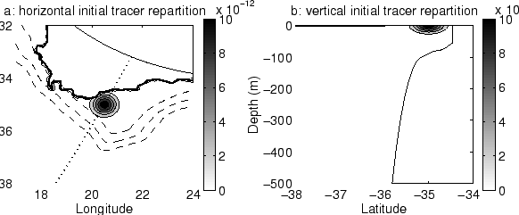 |
In order to explore these physical processes of transport and dispersion, short term
simulations has been conducted, starting from different moments of the long term
simulation, in which a passive tracer, representing the probability of presence of
an
egg, has been introduced into the model. At the beginning of each short term
simulation, the initial value of the tracer 'egg' is defined as a tridimentional
Gaussian patch (figure 3.62):
 |
(110) |
Where  is the radius of the Earth in km,
  is the
latitude,
is the
latitude,  is the latitude of the center of the patch,
  is the longitude,
 is the longitude of the center of the patch,
  is the vertical coordinate in
m, and
is the vertical coordinate in
m, and  is a coefficient set up to obtain
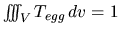 . Hence, only 1 egg is injected into the model at the beginning of each
simulation, with a Gaussian probability of presence to be in a circle of 40 km
radius centered at and , in the 20 first meters from the surface. For
these simulations, the initial patch is centered at
. Hence, only 1 egg is injected into the model at the beginning of each
simulation, with a Gaussian probability of presence to be in a circle of 40 km
radius centered at and , in the 20 first meters from the surface. For
these simulations, the initial patch is centered at  S and
S and  E accounting for an egg spawned on the spawning ground of the western Agulhas Bank
(see Hutchings [1992]). This initial patch is portrayed on figure
(3.62). During the simulation the tracer 'egg' is forced by the
advective and the vertical mixing schemes of the model, employing the
coefficient of vertical mixing of momentum. The open boundaries for this tracer are
passive and radiative to allow its evacuation from the model domain. After the
tracer release, the short term experiments are conducted for 3 months to include all
the whole egg and larvae states for sardines and anchovies. After the larvae state,
the
swimming capabilities of the fishes invalidate the use of a passive tracer to
simulate their behavior.
E accounting for an egg spawned on the spawning ground of the western Agulhas Bank
(see Hutchings [1992]). This initial patch is portrayed on figure
(3.62). During the simulation the tracer 'egg' is forced by the
advective and the vertical mixing schemes of the model, employing the
coefficient of vertical mixing of momentum. The open boundaries for this tracer are
passive and radiative to allow its evacuation from the model domain. After the
tracer release, the short term experiments are conducted for 3 months to include all
the whole egg and larvae states for sardines and anchovies. After the larvae state,
the
swimming capabilities of the fishes invalidate the use of a passive tracer to
simulate their behavior.
Figure 3.63:
Time
series of the tracer surface concentration for an egg released the 1 September of
model year 4. a: after 5 days. b: after 35 days. c: after 65 days. d: after
90 days.
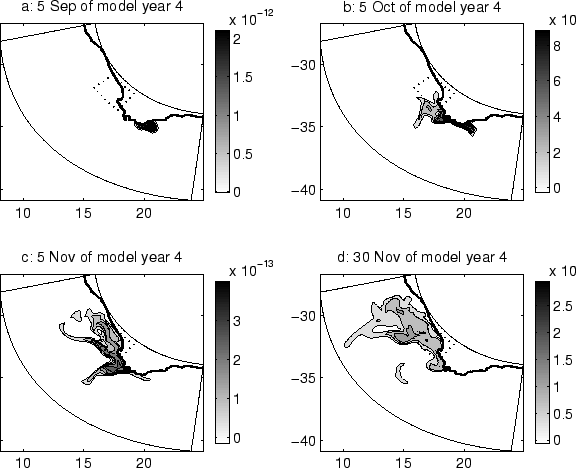 |
The impact of the wind forcing of the transport patterns from the Agulhas Bank to
the Benguela upwelling system is studied by releasing the tracer 'egg' each month of
the summer period, for the low and high resolution experiments, from September of
model year 4 to April of model year 5. A time series of the surface tracer behavior
for
a release just before the upwelling season, the 1 September of model year 4 for the
high resolution experiment is portrayed on figure (3.63). Because
of the important vertical mixing present in the surface mixed layer, the surface
distribution of the tracer is representative of the horizontal repartition for all
the
mixed layer. The averaged wind stress for this period of 3 months is around 0.075
N.m, starting at 0.049 N.m for September and finishing at 0.088
N.m for the end of November. After 5 days, the tracer didn't moved
considerably, sticking to the coast near Cape Agulhas (figure
3.63-a).
After 1 month, a portion of the tracer reaches Cape Columbine, but the core of the
patch
stays near Cape Peninsula. For this period, the patch didn't disperse considerably
(figure 3.63-b). At the beginning of November (figure
3.63-c), the patch has separated into 3 tongues: 1 extending from
Cape
Peninsula due to the presence of an upwelling filament, 1 following the shelf edge
jet
from Cape Columbine, and 1 filling St Helena Bay. At the end of November, the
probability of presence of the egg is approximately uniformly distributed on the
shelf
along the west coast (figure 3.63-d).
Figure 3.64:
Time series of the tracer surface concentration for an egg released the 1
December of model year 4. a: after 5 days. b: after 35 days. c: after 65 days.
d: after 90 days.
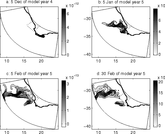 |
Figure (3.64) represents the time series of the tracer evolution for
an egg spawned in the middle of the upwelling season, the 1 December of model
year 4. For this period, the averaged wind stress is 0.085 N.m, starting in
the beginning of December at 0.088 N.m and ending at the end of February at
0.075 N.m. For this simulation, things are going quickly. After 5 days,
the Northern part of the patch has already reached Cape Peninsula (figure
3.64-a). After 1 month, the all of the tracer patch has passed
Cape Peninsula, the effect of the offshore Ekman transport is important with the
major
part of tracer heading north-westward, away from the West Coast. A secondary maximum
of
tracer concentration is trapped around 34 S and 17 E, inside a cyclonic eddy
shed from Cape Peninsula (figure 3.64-b). The effect of the
offshore transport is dramatic after 2 months, for the beginning of February (figure
3.64-c), the largest concentration of tracer is now situated more
than 400 km offshore from the coast. After 3 months, there is almost no chance for a
passive larvae issued from an egg released in December to remain on the shelf along
the
West Coast (figure 3.64-d).
Figure 3.65:
Time
series of the tracer surface concentration for an egg released the 1 March of model
year 5. a: after 5 days. b: after 35 days. c: after 65 days. d: after 90
days.
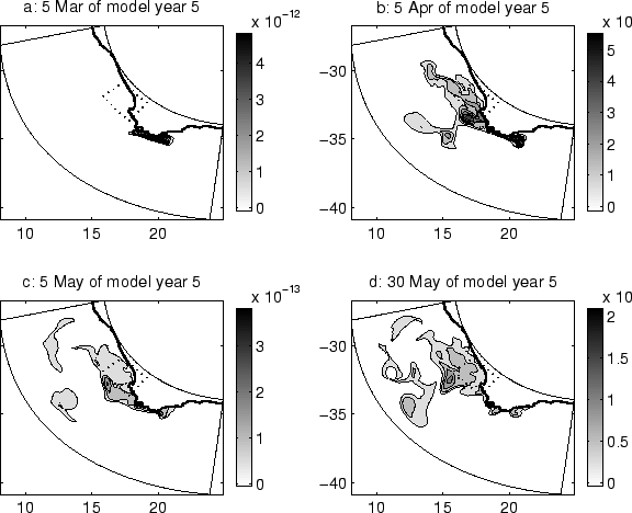 |
For the last time series, the egg is released at the end of the upwelling season,
the 1 March of model year 5. The averaged wind stress along the 3 months of
simulation is 0.045 N.m, starting at 0.075 N.m for the beginning of
March and ending at 0.028 N.m for the end of May. The displacement start
quickly. After 5 days (figure 3.65-a), the pattern is similar as
the previous time series (figure 3.64-a). After 1 month (figure
3.65-b), an important portion of the tracer is already present in St
Helena Bay. There are also 2 patches of tracer that are trapped into cyclonic
eddies
generated from the Cape Peninsula-Cape Columbine area. For the beginning of May,
the
dispersion has slowed down with the diminishing wind stress and few variations are
present between the last 2 months (figures 3.65-c and
3.65-d). After 3 months, the tracer distribution is approximately
equivalent to the end of the case for the release in September (figure
3.63-d).
Figure 3.66:
Time series of the tracer concentration integrated on the volume of the
target zone, in percentage of the total amount of tracer released. Top: for the
low resolution experiment. Bottom: for the high resolution experiment.
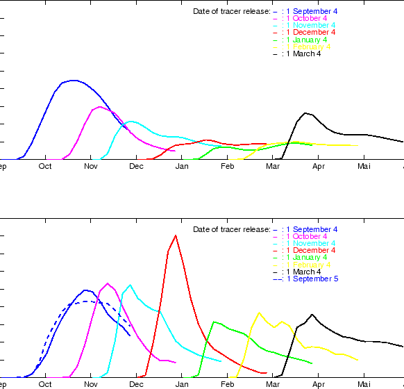 |
To quantify the probability for an egg spawned on the Western Agulhas Bank to reach
the nursery ground of St Helena Bay, time series of the tracer integrated on the
volume limited by the dashed line on figure (3.65) has been
portrayed on figure (3.66). This integrated value accounts for the
probability of the presence in the nursery ground of St Helena Bay of an egg spawned on
the Western Agulhas Bank. For the low resolution experiments, the pattern is clear
(figure 3.66-top). The probability of an egg to reach St Helena Bay
is maximum (almost 25 % chance) if it is released before the upwelling season.
This maximum occurs after around 45 days. The more we advance in the upwelling season,
the more the offshore Ekman transport is active, and the less the eggs have a chance (only 5
% for January) to reach the nursery ground. The chance increases again at the end of
the upwelling season. The time series for the high resolution experiment follows a
more complex pattern (figure 3.66-bottom). For a release in
September the percentage of tracer in the target area follows approximately the same
curve as for the low resolution experiment. For October and November,
the maximum is the same as for September, but the tracer arrives more rapidly
in St. Helena Bay. The tracer is also washed out more quickly from the bay, as we
advance in the upwelling season. For the release in December, the curve differs
dramatically from the low resolution experiment, showing an important amount of
tracer entering the zone in less than a month and leaving the area in also less
than a month. Figure (3.64-b) reveals that this narrow maximum
of tracer in St Helena Bay can be associated with the crossing of the area
by a patch of tracer trapped in a small eddy. This shows that the mesoscale
activity alters considerably the transport pattern from the Agulhas Bank to St Helena
Bay. For the releases of January, February and March, the amount of tracer in St.
Helena Bay follows a relatively constant pattern: rapid increase to reach a maximum
of 15 % after less than 1 month and slow decrease. The impact of the interannual
variability observed in the outputs of the high resolution experiment is tested
for the transport of eggs by making the comparison between an experiment for an
egg released the 1 September of model year 5 and the experiment for an egged
release the 1 September of model year 4. The dashed line on figure
(3.66) reveals that although a certain degree of interannual
variability is present in the model outputs, the global transport patterns do not
differ dramatically from one year to the other. This allows sardines and anchovies
to adapt their reproductive strategies to these relatively stable global transport
patterns. One can note that differences in the transport behavior between the low
resolution and the high resolution experiments occur principally during the
upwelling season, when the mesoscale activity along the west coast is the strongest.
This result connects to the conclusion of the second chapter that shows that during
the upwelling season, although the Ekman transport can carry the material away from the
coast, eddies can trap it for a certain amount of time in the coastal domain.
In this chapter, a primitive equation model, the Regional Oceanic Model Systems, has
been configured to reproduce the characteristic patterns of the circulation around
the South-western corner of Africa. The model resolves the free surface,
hydrostatic,
tri-dimensional primitive equations featuring high order schemes and new
parameterizations over variable topography using stretched, terrain following
coordinates. The horizontal, orthogonal, curvilinear grid has been designed in a
pie
shape to fit the curve of the South African coastline. Specific open boundary
conditions involving a radiative one way nesting of seasonal time averaged data from
a large scale oceanic model allow long term stable simulations. Two
configurations are set up: a low resolution one with a grid space ranging from 18 km
to 31 km and a high resolution one with a grid space ranging from 9 km to 16 km. The
surface fluxes are derived from the coarse monthly climatology of the COADS dataset.
After a spin-up of 2 years, the model has reached a statistical equilibrium. The
high resolution experiment produces important intrinsic instabilities associated with
the upwelling process and the Agulhas Current dynamics, with formation of plumes,
filaments and eddies. For the low resolution experiment, whereas on a large scale
the time averaged circulation, temperature and salinity compares to the
observations, some aspects of the solution such as the Agulhas Current retroflection
or the coastal circulation are not correctly represented. In the high resolution
case, the solution is much more satisfactory and compares quantitatively to the
known circulation. The volume averaged level of kinetic
energy is higher than for the low resolution experiment due to the better resolved
mesoscale processes. The averaged position of the retroflection of the Agulhas
Current now corresponds to the observations, and important aspects of the coastal
circulation such as the coastal jets are now properly resolved. The signature of the
Agulhas Current is still present at 1000 m depth. At this depth and below, the
circulation in the Benguela is slow, meandering and principally poleward. The
depth integrated transport for the Benguela is ranging from 10 to 20 Sv and is more
than 60 Sv for the Agulhas Current, in agreement with previous studies. The time
averaged sea surface temperature compares quantitatively to satellite data. The
principal difference is the stronger upwelling observed in the model outputs. This
can be related to the low resolution dataset employed for the wind forcing. The
bottom temperature and salinity values stay in reasonable agreement with long term
observations.
The length of the experiment allows a statistic analysis of the variability. The sea
surface temperature variance shows a maximum on the Agulhas Bank where the currents
are weak and a minimum in St Helena Bay where the presence of the upwelling plume
seems to balance the seasonal variations. This pattern is quantitatively confirmed
by sea surface satellite data. The root mean square of sea surface height is
compared to altimeter data. It reveals both in model and data a maximum in
variability in the Agulhas retroflection area and minimums on the shelves along the
South and the West coasts. The same pattern is observed from the subsurface eddy
kinetic energy. Although the modelized EKE compares quantitatively to data north of
35 S, where the variability is produced in-situ, an important difference is
noticeable in the area influenced by the Agulhas Current. This discrepancy can be
explained by the smooth time averaged data used to generate the Agulhas current at
the Eastern boundary and by the constrain generated by the western boundary on the
spawning off the Agulhas rings. This difference is confirmed by the ellipses of
subsurface velocity variance. They also reveals an important anisotropy of the
variability near Cape Columbine, near Cape Peninsula and South of the Agulhas Bank.
These area of anisotropy in variability are also the preferred area for eddy
generation. Important anisotropy in variability is also present along the open
boundaries which tend to minimize the cross boundary variability.
Although the wind forcing is coarse in space and time, the modelized upwelling
system of the west coast shows important features such as the upwelling plume of
Cape Columbine, the Namaqualand upwelling center, the upwelling eddies
generated by the major capes, and the filaments spreading from the main upwelling
front. This shows that the temporal and spatial small scale structures of the wind
field are not the primary generators of the mesoscale activity of the upwelling
system. It is rather induced by intrinsic instability processes. On the shelves, the
time averaged circulation is highly controlled by the topography. A part of the
Agulhas Current tends to follow the western part of the Agulhas Bank to feed the
Good Hope jet. A surface equatorward baroclinic jet follows the shelf edge and a
poleward undercurrent flows along the shelf break. The subsurface coastal counter
current is present in the high resolution simulation. Standing coastal wave patterns
can be noticed in St Helena Bay, in agreement with the analysis of the second
chapter, but the treatment of the topography induces a steepening of the shelf,
inhibiting the generation of a cyclonic mean circulation in the bay.
Mesoscale processes in association to the Agulhas Current are also simulated by the
model. They include:
- Cyclonic eddies that are shed from the southern tip of the Agulhas bank,
where the Agulhas Current detaches from the topographic control.
- Shear edge eddies that are formed on the eastern Agulhas Bank, where the
Agulhas Current overshoots the concave part of the shelf break.
This analysis of the model outputs gives confidence in the validity of the
simulation. A set of experiments has been set up to study the transport patterns of
sardines and anchovies from the spawning area of the western Agulhas Bank to the
nursery ground of St Helena Bay. A passive tracer has been released at different
times of the simulation. Each `tracer simulation' has been conducted for 3 months.
The amount of tracer that manages to reach St Helena Bay is highly dependent on the
date of the release. If the tracer release occurs before the upwelling season, it
fills slowly St. Helena Bay. An important portion of tracer is still along the West
Coast after 3 months. On the contrary, if the tracer release is done during the
upwelling season, though the tracer arrives very quickly in the West Coast, it is
also rapidly carried away by the Ekman transport. If the release occurs after the
upwelling season the amount of tracer in St. Helena Bay increases again. During the
upwelling season, the loss of tracer is more important for the low resolution
experiment than for the high resolution experiment. This reveals that the mesoscale
activity is able to counter the effects of the offshore Ekman transport, or that the
along shore jets responsible of transport are not well reproduced for the low
resolution experiment.
Here is the end of the manuscript, the time to take the stock of what has been
achieved during this project. The goals of the PhD were
- to study the dynamics of mesoscale processes related to retention within the St
Helena Bay nursery ground
- to develop a high resolution regional model to simulate the shelf circulation
along the South and West coasts of South Africa.
The work could have been focused on the design of a
3D realistic model or on the study of a particular process of the system. The
step by step approach chosen was more general: starting with a description of
the system that has led to the selection of a few processes, concentrating
on a specific process in St Helena Bay using both numerical and analytical
approaches, and ending by a realistic simulation of the circulation of the
Southern Benguela.
The barotropic study reveals that a wind driven equatorward current can
generate a standing process in the lee of a cape. In the case of St Helena Bay,
the numerical study shows that this process should take the form of a standing
cyclonic eddy, controlled by a balance between advection and bottom friction. A
length scale derived from this balance, which can be considered as an
e-folding length scale, can then predict the size of the eddy as a function of
the wind stress and the bottom friction parameter. Sensitivity tests reveal
some discrepancies between this length scale and the size of the eddy,
especially for smaller capes where the slope in the bay has gained importance.
In the presence of bottom slope, standing shelf waves are more likely to develop.
An analytical study shows that standing shelf waves can be excited by a mean
current past a cape. The tracer, representing the age of the water, has
been introduced in the model. It exhibits the retention induced by the standing
recirculation process. Upwelling favorable winds can generate currents
responsible for eggs and larvae dispersion. But, at the same time, these currents
can induce recirculation in the lee of capes like Cape Columbine that can trap
eggs and larvae in a favorable environment.
The particularity of the Benguela system, with the Agulhas Current retroflecting
just South of the area of interest did not facilitate the implementation of a
realist 3-D model of the region. Tests have been conducted using a low
resolution configuration to set-up the open boundary conditions. The treatment
of the bottom topography for this simulation gave an incorrect representation
of the shelf circulation and the detachment of the Agulhas Current. For the
high resolution experiment the solution is more satisfactory, and compares
with observations for most of the processes. They include:
- The localized upwelling centers of Cape Peninsula, Cape Columbine,
Namaqualand and Lüderitz.
- The upwelling eddies that are shed from the Cape Peninsula and Cape
Columbine
- The upwelling plume that extend from Cape Columbine
- The filaments that extends from the upwelling front
- The equatorward baroclinic jet associated with the upwelling front
- The Columbine divide
- The poleward subsurface counter-current and the poleward undercurrent
along the shelf break
- The poleward deep motion along the slope
- The weak circulation on the Agulhas Bank
- The convergent currents on the western margin of the Agulhas Bank that
feed the Good Hope jet
- The cyclonic eddies shed from the Agulhas Current in the lee of the
Agulhas Bank
- The shear edge eddies along the eastern and southern part of the Agulhas
Bank
- The Agulhas retroflection
The major ingredients of Southern Benguela are present in the simulation. It is the
first time that these local processes, described in numerous publications, have been
modelized with this level of accuracy.
Although the surface forcing is derived from a smooth monthly climatology, the
mesoscale activity generates a significant high frequency variability.
Its amplitude along the West Coast of South Africa compares quantitatively with
observations. This result shows that the variability along the West Coast is
more a consequence of intrinsic instability of the coastal ocean rather than
a direct forcing from small scale wind variations.
Some differences have also been noticed when comparing model results with data:
- The time-averaged modelized sea surface temperature along a coastal
narrow band North of Cape Columbine is 2 to 3 C smaller than the
temperature observed from satellite imagery. It has been observed that the intensity of
upwelling favorable wind stress is smaller along the coast North of Cape
Columbine [Jury, 1988], but this pattern is not present in the dataset used to
force the model. This can explain the difference between the model and the
observations.
- The subsurface eddy kinetic energy is 2 times smaller than the eddy
kinetic energy derived from altimeter data in the Agulhas retroflection area.
There is 2 possible causes for this difference. Firstly, the Agulhas Current
shows important variations that are generated upstream of the model domain and
propagate with the flow, like the Natal pulses [De Ruijter et al., 1999a,Lutjeharms and Roberts, 1988]. The
seasonal time-averaged data set employed to force the Agulhas Current at the
eastern open boundary does not inject this non-local variability into the model.
Secondly, the western open boundary is close to the retroflection area and mights
affect the Agulhas rings generation process.
- The cyclonic weak motion observed in St Helena Bay and analyzed in the
second chapter is not present in the realistic model outputs. The treatment of
bottom topography for this level of resolution enhanced the slope of the shelf,
inhibiting the possible generation of this standing process.
A tracer, representing the probability of presence of an egg spawned on
the western Agulhas Bank has been introduced to simulate the transport patterns
between the Agulhas Bank and the West Coast of South Africa. It shows the negative
effect of the upwelling favorable wind for the transfer from the Agulhas Bank to
the West Coast and the positive effect of the mesoscale eddies and jet on the
retention of the biological materials in the favorable areas. This is in agreement
with the last result of the second chapter.
Prospects
- The realistic 3D model has been developed in order to produce an accurate
portrayal of the dynamics of the Southern Benguela to study the impact of the
environment on the recruitment of small pelagics. An individual based model (IBM)
has been developed by the VIBES group. This model allows the simulation of the path
of fish eggs, larvae and juveniles when they are released in the model domain. The
coupling of the IBM with the results of the physical model allows the simulation and
analysis of transport processes affecting the recruitment of sardines and anchovies in
the Southern Benguela. Specific scenarios (like strong upwelling or weak upwelling)
can be undertaken to understand the impact of the variability of the environment on
the living resources. The coupling of a coastal ocean model to an IBM constitutes
a powerful tool for the understanding of ecosystem dynamics. This technique has
been successfully applied to quantify the effects of advection on pollock larvae in
Alaska [Hermann et al., 1996] and on cod and haddock larvae on George Bank [Werner et al., 1993].
- In the second chapter, we have shown the generation of a standing process in
the barotropic case. Is it still valid when stratification is taken into account ?
The comparison of the results with the observed circulation in St Helena Bay seems
to maintain this hypothesis, but the advection by a mean current is not clear in
the baroclinic case.
- The realistic model provides a large amount of information and specific
processes that can been studied from the model outputs. The forcing of the poleward
undercurrent and counter-current can be diagnosed by computing the different terms
of the momentum and vorticity equations from the model outputs.
Special attention can be given to the de-stabilization processes of the upwelling
front along the West Coast of South Africa. The quantification of energy
transformation mechanisms can lead to the indication of the type of instability
process that is responsible of the de-stabilization of the front.
- Simplified models and analytical analysis, inspired by the work of Gill and
Schumann [1979], of the shear edge eddies obtained on the Agulhas Bight could
explain the reason for these recurrent features. This process should be also present
on the coastal side of the other western boundary currents.
- The analysis of the results of the high resolution experiment allows us to
identify directions to follow in the future, in order to improve the quality of the
realistic simulation:
- The topography on the shelf near Cape Peninsula and in St Helena Bay
has been significantly altered during the smoothing process. The 100 m
isobath passes through the Cape Peninsula and the exaggerated slope of the shelf in St
Helena Bay can inhibit the generation of the cyclonic process, important for the
retention of biological material in the coastal area. The algorithm of topography
smoothing can be corrected in order to respect the general shape of the shelves.
Simulation with higher spatial resolution can allow the use of a more realistic
bottom topography, but at a larger numerical cost. A new pressure gradient scheme
is still in development at UCLA [Shchepetkin and McWilliams, in preparation]. If this formulation gives the
results expected, it could be possible to employ a more accurate bottom topography
at the actual level of resolution.
- The shedding of the Agulhas rings seems to have been constricted by
the vicinity of the eastern open boundary. This boundary should be placed at a few
hundred of kilometers offshore in order to allow a greater degree of freedom for the
detachment of the Agulhas rings.
- The level of eddy kinetic energy in the Agulhas area is 2 times
smaller for the model than for the observations. Although an important source of
variability for the Agulhas Current has been recognized to be the Mozambique
channel [Biastoch and Krauß, 1999], thousands of km upstream of our domain, the displacement of
the western boundary around 28 E, where the Agulhas Current appears to be more
stable, should enhance the simulation of the variability in the retroflection area.
Another possibility could be the utilization of the direct outputs of AGAPE
instead of using a seasonal climatology. In this case, the larger amount of data
that should have to be treated to fit to the regional model grid dramatically increases
the numerical cost of the preprocessing chain. We will rapidly reach
the paradox that more cpu time should be necessary to prepare the experiments than
to actually run them. In this case, in order to obtain a meaningful solution, it
should be also necessary to enforce the compatibility of the surface forcing
between the regional model and the AGAPE basin scale model.
- A finer climatological dataset can be derived for the surface wind
forcing to obtain a sea surface temperature closer to the observations along the
west coast.
- Test experiments with low wind forcing, high wind forcing, warm water
intrusion from the North, or using a more variable wind stress can allow the
quantification of the response of the Benguela upwelling system on the interannual
variability of the external forcing. This response can dramatically affect the
recruitment.
- The use of realistic surface forcing and the comparison with the simulation
obtained in the present work can give a quantification of the direct impact of the
surface
forcing on the variability of the Benguela system.
- The use of embedded grids, in one way and in two ways, can resolve one of the
most important problem of coastal dynamics: the need for a high resolution solution
in the coastal domain in opposition to the need for a proper representation of the
effects induced by the large scale circulation. This method can be useful for the
inclusion of processes such as the variability produced by eddies generated as far
as the Mozambique Channel. Using these methods, it will also be possible to have
fine scale high resolution subgrids for the areas of interest such as bays like St.
Helena Bay, Saldanha Bay, or False Bay. It opens a wide field of non-academic
applications of the model solution for coastal management, harbor and industrial
installations, or pollutant dispersion studies.
Many other improvements can be added to the actual model to produce a better
representation of the Benguela ecosystem, such as the assimilation of data, the
introduction of tides, the modeling of the river outflows, or the modeling
of the primary production... Each increase of the complexity of the modelized
system, will result in an increase of the complexity of the solution. New tools
should then be designed to help the understanding of the key processes that are
structuring these solutions. Recently, an important effort has been conducted to
understand the dynamics of coastal ecosystems, an example is the work conducted for
the West Coast of the United States [Miller et al., 1999]. The experience gained and the
tools designed for the study of the Benguela ecosystem could be applied to other
coastal domains of the world. Important fundamental insight could
be obtained by comparing the dynamics of the different domains.
- Bailey and Chapman, 1985
-
Bailey, G. W., and P. Chapman,
The nutrient status of the St. Helena bay region in February 1979,
In South African Ocean Colour Experiment,
edited by L.V. Shannon,
pp. 125-145,
Sea Fisheries Research Institute,
Cape Town,
1985.
- Bakun, 1996
-
Bakun, A.,
Patterns in the Ocean: Ocean Processes and Marine Population Dynamics,
323 pp,
University of California Sea Grant,
San Diego,
Calif.,
USA,
1996.
- Bakun, 1998
-
Bakun, A.,
Ocean triads and radical interdecadal stock variability: bane
and boon for fisheries management,
In Reinventing fisheries management,
edited by T. Pitcher, P.J.B. Hart and D. Pauly,
pp. 331-358,
Chapman and Hall,
London,
1998.
- Ball, 1967
-
Ball, F. K.,
Edge waves in an ocean of finite depth,
Deep-Sea Res.,
14,
79-88,
1967.
- Barnier et al., 1998
-
Barnier, B., P. Marchessiello, A. Pimenta de Miranda,
J. M. Molines, and M. Coulibaly,
A sigma-coordinate primitive equation model for studying
the South Atlantic. Part I: model configuration with
error estimates,
Deep-Sea Res.,
45,
543-572,
1998.
- Bathmann et al., 1994
-
Bathmann, U., V. Smetacek, H. de Baar, E., Farbach, and G. Krause,
The expeditions ANTARKTIS X/6-8 of the research vessel
"Polarstern" in 1992/93,
Rep. Polar Res.,
135,
241 pp,
1994.
- Batteen, 1997
-
Batteen, M. L.,
Wind-forced modeling studies of currents, meanders, and
eddies in the California Current system,
J. Geophys. Res.,
102,
985-1010,
1997.
- Beal and Bryden, 1997
-
Beal, L. M., and H. L. Bryden,
Obervations of an Agulhas undercurrent,
Deep-Sea Res. I,
44,
1715-1724,
1997.
- Becker, 1991
-
Becker, A.,
The separated flow past a cylinder in a rotating frame,
J. Fluid Mech.,
224,
117-132,
1991.
- Biastoch, 1998
-
Biastoch, A.,
Zirkulation und Dynamik in der Agulhasregion anhand eines numerischen Modells,
Berichte aus dem Institut für Meereskunde an der
Christian-Albrechts-Universität,
Kiel,
301,
118 pp,
1998.
- Biastoch and Krauß, 1999
- Biastoch, A., and W.
Krauß,
The Role of Mesoscale Eddies in the Source Regions of
the Agulhas Current,
J. Phys. Oceanogr.,
29,
2303-2317,
1999.
- Boyd and Hewitson, 1983
-
Boyd, A. J., and J. D. Hewitson,
Distribution of anchovy larvae of the west coast of southern Africa between
 and
and  S, 1979-1983,
S. Afr. J. mar. Sci.,
1,
71-75,
1983.
S, 1979-1983,
S. Afr. J. mar. Sci.,
1,
71-75,
1983.
- Boyd and Oberholster, 1994
-
Boyd, A. J., and G. P. J. Oberholster,
Currents offf the West and South coasts of
South Africa,
SA Shipping News & Fishing Industry Review,
26-28,
1994.
- Boyd and Shilligton, 1994
-
Boyd, A. J., and F. A. Shilligton,
Physical forcing and circulation patterns on the Agulhas Bank,
S. Afr. J. Sci.,
90,
114-122,
1994.
- Boyd and Nelson, 1998
-
Boyd, A. J., and G. Nelson,
Variabiliy of the Benguela current off the Cape Peninsula, South Africa,
S. Afr. J. mar. Sci.,
19,
15-39,
1998.
- Boyer and Tao, 1987
-
Boyer, D. L., and L. Tao,
On the motion of linearly stratified rotating
fluids past capes,
J. Fluid Mech.,
180,
429-449,
1987.
- Boyer et al., 1987
-
Boyer, D. L., Cheng R., Chabert D'Hières G., and Didelle H.,
On the formation of vortices from side-wall mounted
obstacles in rotating systems,
Dyn. Atmos. Oceans,
11,
59-86,
1987.
- Brink, 1991
-
Brink, K. H.,
Coastal-trapped waves and wind-driven currents
over the continental shelf,
Annu. Rev. Fluid Mech.,
23,
389-412,
1991.
- Brink, 1998
-
Brink, K. H.,
Wind-driven currents over the continental shelf,
In The Sea,
Vol. 10,
The Global Coastal Ocean: Processes and Methods,
edited by K.H. Brink and A.R. Robinson,
pp. 3-20,
Wiley,
New York,
1998.
- Brundrit, 1981
-
Brundrit, G. B.,
Upwelling fronts in the southern Benguela region,
Trans. Roy. Soc. S. Afr.,
44,
309-313,
1981.
- Brundrit et al., 1987
-
Brundrit, G. B., B. A. de Cuevas, and A. M. Shipley,
Long-term sea-level variability in the eastern
south Atlantic and comparison with that eastern
Pacific,
S. Afr. J. mar. Sci.,
5,
73-78,
1987.
- Buchwald and Adams, 1968
-
Buchwald, V. T., and J. K. Adams,
The propagation of continental shelf waves,
Proc. Roy. Soc. A.,
305,
235-250,
1968.
- Christensen, 1980
-
Christensen, M. S.,
Sea-surface temperature charts for Southern Africa, south of 26°S,
S. Afr. J. Sci.,
76,
541-546,
1980.
- Clark and Brink, 1985
-
Clark, A. J., and K. H. Brink, The response of stratified, frictional
flow of shelf and slope waters to fluctuating large-scale, low-frequency wind
forcing,
J. Phys. Oceanogr.,
15,
439-493,
1985.
- Csanady, 1978
-
Csanady, G. T., The arrested topographic wave,
J. Phys. Oceanogr.,
8,
47-62,
1978.
- Csanady, 1982
-
Csanady, G. T.,
Circulation in the Coastal Ocean,
279 pp,
D. Reidel Publishing Company,
Dordrecht,
1982.
- Csanady, 1998
-
Csanady, G. T.,
The non-wavelike response of a continental shelf to wind,
J. Mar. Res.,
56,
773-788,
1998.
- Crepon et al., 1984
-
Crepon M., C. Richez, and M. Chartier,
Effects of Coastline Geometry on Upwellings,
J. Phys. Oceanogr.,
14,
1365-1382,
1984.
- Cury and Roy, 1989
-
Cury P., and C. Roy,
Optimal environmental window and pelagic fish
recruitment success in upwelling areas,
Can. J. Fish. Aquat. Sci.,
46,
670-680,
1989.
- Cury et al., 1995
-
Cury, P., C. Roy, R. Mendelssohn, A. Bakun, and D. M. Husby,
Moderate is better: exploring nonlinear climatic effect on the
Californian northern anchovy,
Can. Spec. Publ. Fish. Aquat. Sci.,
121,
41-424,
1995.
- Da Silva et al., 1994
-
Da Silva, A. M., C. C. Young, and S. Levitus,
Atlas of surface marine data 1994,
volume 1,
algorithms and procedures,
74 pp.,
NOAA Atlas NESDIS 6,
U. S. Department of Commerce,
NOAA,
NESDIS,
USA,
1994.
- Davies et al., 1990
-
Davies, P. A., P. Besley, D. L. Boyer,
An experimental study of flow past a triangular cape
in a linearly stratified fluid,
Dyn. Atmos. Oceans,
8,
497-528,
1990.
- De Ruijter et al., 1999a
-
De Ruijter, W. P. M., P. J. van Leeuwen, and J. R. E. Lutjeharms,
Generation and evolution of Natal Pulses: solitary meanders in the Agulhas
Current,
J. Phys. Oceanogr.,
29,
3043-3055,
1999a.
- De Ruijter et al., 1999b
-
De Ruijter, W. P. M., A. Biastoch, S. S. Drijfhout,
J. R. E. Lutjeharms, R. P. Matano, T. Pichevin,
P. J. van Leeuwen, and W. Weijer, 1999:
Indian-Atlantic inter-ocean exchange: dynamics,
estimation and impact.
J. Geophys. Res.,
104,
20885 - 20911,
1999b.
- Dingle and Nelson, 1993
-
Dingle, R. V., and G. Nelson,
Sea-bottom temperature, salinity and dissolved
oxygen on the continental margin off south-western
Africa,
S. Afr. J. mar. Sci.,
13,
33-49,
1993.
- Ducet et al., 2000
-
Ducet, N., P.-Y. Le Traon, and G. Reverdin,
Global high resolution mapping of ocean circulation from T/P end ERS-1/2,
J. Geophys. Res.,
105,
19477-19498,
2000.
- Duncombe Rae et al., 1996
-
Duncombe Rae, C. M., S. L. Garzoli, and A. L. Gordon,
The eddy field of the South-East Atlantic Ocean:
a statistical census from the BEST project,
J. Geophys. Res.,
101,
11949 - 11964,
1996.
- Durand et al., 1998
-
Durand, M.-H., P. Cury, R. Mendelssohn,
C. Roy, A. Bakun, and D. Pauly,
Global versus local changes in upwelling systems,
558 pp,
Editions ORSTOM,
Paris,
1998.
- Enriquez and Friehe, 1995
-
Enriquez, A. G., and C. A. Friehe,
Effects of wind stress and wind stress curl variability
on coastal upwelling,
J. Phys. Oceanogr.,
25,
1651-1671,
1995.
- Flather, 1976
-
Flather, R. A.,
A tidal model of the northwest European continental shelf,
Mem. Soc. R. Sci. Liège,
10,
141-164,
1976.
- Fowler and Boyd, 1998
-
Fowler, J. L., and A. J. Boyd,
Transport of anchovy and sardine eggs and larvae from the western Agulhas Bank
to the West Coast during the 1993/94 and 1994/95 spawning seasons,
S. Afr. J. mar. Sci.,
19,
181-195,
1998.
- Garzoli and Gordon, 1996
-
Garzoli, S. L., and A. L. Gordon,
Origins and variability of the Benguela current,
J. Geophys. Res.,
101,
897-906,
1996.
- Gill and Schumann, 1974
-
Gill, A. E., and E. H. Schumann,
The generation of long shelf waves by the wind,
J. Phys. Oceanogr.,
4,
83-90,
1974.
- Gill and Schumann, 1979
-
Gill, A. E., and E. H. Schumann,
Topographically induced changes in the structure of an inertial coastal jet:
application to the Agulhas Current,
J. Phys. Oceanogr.,
9,
975-991,
1979.
- Goschen and Schumann, 1990
-
Goschen, W. S., and E. H. Schumann,
Agulhas Current variability and inshore structures off the Cape
Province, South Africa,
J. Geophys. Res.,
95,
667-678,
1990.
- Goschen and Schumann, 1994
-
Goschen, W. S., and E. H. Schumann,
An Agulhas Current intrusion into Algoa Bay during August 1988,
S. Afr. J. Mar. Sci.,
14,
47-57,
1994.
- Graham and Largier, 1997
-
Graham, W. M., and J. L. Largier,
Upwelling shadows as nearshore retention sites: the example of northern
Monterey Bay,
Cont. Shelf Res.,
17,
509-532,
1997.
- Gründlingh, 1979
-
Gründlingh, M. L.,
Observation of a large meander in the Agulhas Current.
J. Geophys. Res.,
84,
3776-3778,
1979.
- Gründlingh, 1983
-
Gründlingh, M. L.,
On the course of the Agulhas Current.
S. Afri. Geogr. J.,
65,
49-57,
1983.
- Gründlingh and Pearce, 1990
-
Gründlingh, M. L., and A. F. Pearce,
Frontal features of the Agulhas Current in the Natal Bight.
S. Afr. Geogr. J.,
72,
11-14,
1990.
- Gründlingh, 1995
-
Gründlingh, M. L., 1995:
Tracking eddies in the southeast Atlantic and southwest Indian oceans with
TOPEX/POSEIDON.
J. Geophys. Res.,
100,
24977-24986,
1995.
- Haidvogel et al., 1991
-
Haidvogel, D .B., A. Beckmann, and K. S. Hedström,
Dynamical simulations of filament formation and evolution
in the coastal transition zone,
J. Geophys. Res.,
96,
15,017-15,040,
1991.
- Haidvogel et al., 2000
-
Haidvogel, D. B., H. G. Arango, K. S. Hedström, A. Beckmann, P.
Malanotte-Rizzoli, and A. F. Shchepetkin,
Model evaluation experiments in the North Atlantic Basin: simulations in
nonlinear terrain-following coordinates,
Dyn. Atm. Oceans,
32,
239-281,
2000.
- Haney, 1991
-
Haney, R. L.,
On the pressure force over steep
topography in sigma coordinate Ocean models,
J. Phys. Oceanogr.,
21,
610-619,
1991.
- Harris et al., 1978
-
Harris, T. F. W., R. Legeckis, and D. van Foreest,
Satellite infra-red images in the Agulhas Current system.
Deep-Sea Res.,
25,
543-548,
1978.
- Hedström, 1997
-
Hedström, K. S.,
User's Manual for an S-Coordinate Primitive Equation
Ocean Circulation Model (SCRUM) Version 3.0,
116 pp,
Institute of Marine and Coastal Sciences,
Rutgers University,
USA,
1997.
- Hermann et al., 1996
-
Hermann, A. J., W. C. Ruggen, P. J. Stabeno, and N. A. Bond,
Physical transport of young pollock larvae (Theragra chalcogramma) near
Shelikof Strait as inferred from a hydrodynamic model,
Fish. Oceanogr.,
5,
58-70,
1996.
- Hjort, 1914
-
Hjort, J.,
Fluctuations in the great fisheries of Northern Europe,
Rapp. P.-v. Réun. Cons. Perm. Int. Explor. Mer.,
19,
1-228,
1914.
- Hjort, 1926
-
Hjort, J.,
Fluctuations in the year classes of important food,
fishes. J. Cons. Int. Explor. Mer.,
1,
5-38,
1926.
- Holden, 1985
-
Holden, C. J.,
Currents in St. Helena Bay inferred from radio-tracked drifters,
In South African Ocean Colour Experiment,
edited by L.V. Shannon,
pp. 97-109,
Sea Fisheries Research Institute,
Cape Town,
1985.
- Hutchings, 1992
-
Hutchings, L., Fish harvesting in a variable, productive environment,
S. Afr. J. mar. Sci.,
12,
297-318,
1992.
- Hutchings et al., 1998
-
Hutchings, L., M. Barange, S. F. Bloomer, A. J. Boyd, R. J. M. Crawford,
J. A. Hugget, M. Kerstan, J. L. Korrubel, J. a. De Oliviera, S. J. Painting,
A. J. Richardson, L. J. Shannon, F. H. Schulein, C. D. Van de Lingen,
and H. M. Verheye,
Multiple factors affecting South African anchovy
recruitment in the spawning, transport and nursery areas,
S. Afr. J. mar. Sci.,
19,
211-225,
1998.
- Huthnance, 1975
-
Huthnance, J. M.,
On trapped waves over a continental shelf,
J. Fluid Mech.,
69,
689-704,
1975.
- Huthnance, 1978
-
Huthnance, J. M.,
On coastal trapped waves: analysis and numerical
calculation by inverse iteration,
J. Phys. Oceanogr.,
8,
74-92,
1978.
- Huthnance, 1981
-
Huthnance, J. M.,
Waves and currents near the continental shelf edge,
Prog. Oceanog.,
10,
193-226,
1981.
- Jury, 1985a
-
Jury, M. R.,
Case studies of alongshore variations in wind-driven upwelling in the southern
Benguela region,
In South African Ocean Colour Experiment,
edited by L.V. Shannon,
pp. 29-46,
Sea Fisheries Research Institute,
Cape Town,
1985.
- Jury, 1985b
-
Jury, M. R., Mesoscale variations in summer winds over the Cape
Columbine -St. Helena Bay region, South Africa,
S. Afr. J. mar. Sci.,
3,
77-88,
1985.
- Jury, 1986
-
Jury, M. R.,
The sudden decay of upwelling off the cape peninsula,
South Africa: a case study,
S. Afr. J. mar. Sci.,
4,
111-118,
1986.
- Jury, 1988
-
Jury, M. R.,
Case studies of the response and spatial distribution
of wind-driven upwelling off the coast of Africa:
 south,
Cont. Shelf Res.,
8,
1257-1271,
1988.
south,
Cont. Shelf Res.,
8,
1257-1271,
1988.
- Jury and Taunton-Clark, 1986
-
Jury, M. R., and J. Taunton-Clark,
Wind-driven upwelling off the Namaqualand coast
of South Africa in spring 1980,
S. Afr. J. mar. Sci.,
4,
103-110,
1986.
- Jury and Brundrit, 1992
-
Jury, M. R., and G. B. Brundrit,
Temporal organization of upwelling in the
southern Benguela ecosystem by resonant coastal
trapped waves in the ocean and atmosphere,
S. Afr. J. mar. Sci.,
12,
219-224,
1992.
- Jury et al., 1985
-
Jury, M. R., F. Kamstra, and J. Taunton-Clark,
Synoptic summer wind cycles and upwelling off
the southern portion of the Cape Peninsula,
S. Afr. J. mar. Sci.,
3,
33-42,
1985.
- Jury et al., 1990
-
Jury, M. R., C. I. McArthur, and G. B. Brundrit,
Pulsing of the Benguela upwelling region: large-scale
atmospheric controls,
S. Afr. J. mar. Sci.,
9,
27-41,
1990.
- Kamstra, 1985
-
Kamstra, F.,
Environmental features of the southern Benguela with
special reference to the wind stress,
In South African Ocean Colour Experiment,
edited by L.V. Shannon,
pp. 13-27,
Sea Fisheries Research Institute,
Cape Town,
1985.
- Kliem and Pietrzak, 1999
-
Kliem, N., and J. D. Pietrzak,
On the pressure gradient error in sigma coordinate
ocean models: A comparison with a laboratory experiment,
J. Geophys. Res.,
104,
29,781-29,799,
1999.
- Klinger, 1993
-
Klinger, B. A.,
Gyre formation at a corner by rotating barotropic
coastal flows along a slope,
Dyn. Atmos. Oceans,
19,
27-63,
1993.
- Klinger, 1994
-
Klinger, B. A.,
Inviscid current separation from rounded capes,
J. Phys. Oceanogr.,
24,
1805-1811,
1994.
- Kundu, 1990
-
Kundu, P. K.,
Fluid Mechanics,
629 pp.,
Academic Press,
San Diego,
Calif.,
1990.
- Lamberth and Nelson, 1987
-
Lamberth, R., and Nelson G., Field and analytical drogue studies
applicable to the St. Helena bay area off South Africa's west coast,
S. Afr. J. mar. Sci.,
5,
163-169,
1987.
- Large et al., 1994
-
Large, W. G., J. C. McWilliams, and S. C. Doney,
Oceanic vertical mixing: a review and a model
with a nonlocal boundary layer parameterization,
Rev. Geophys.,
32,
363-403,
1994.
- Levitus, 1982
-
Levitus, S.,
Climatological Atlas of the World Ocean,
Professional Paper 13,
173 pp.,
NOAA,
USA,
1982.
- Lightill, 1967
-
Lightill, M. J.,
On waves generated in dispersive systems by travelling
forcing effects, with applications to the dynamics of
rotating fluids,
J. Fluid Mech.,
27,
725-752,
1967.
- Lutjeharms, 1981
-
Lutjeharms, J. R. E.,
Features of the southern Agulhas Current circulation from satellite remote
sensing,
S. Afr. J. Sci.,
77,
231-236,
1981.
- Lutjeharms and Stockton, 1987
-
Lutjeharms, J. R. E., and P. L. Stockton,
Kinematics of the upwelling front off southern Africa,
S. Afr. J. mar. Sci.,
5,
35-49,
1987.
- Lutjeharms and Roberts, 1988
-
Lutjeharms, J. R. E., and H. R. Roberts,
The Natal pulse; an extreme transient on the Agulhas Current,
J . Geophys. Res.,
93,
631-645,
1988.
- Lutjeharms and Valentine, 1988
-
Lutjeharms, J. R. E., and H. R. Valentine,
Evidence for persistent Agulhas rings south-west of Cape Town,
S. Afr. J. Sci.,
84,
781-783,
1988.
- Lutjeharms and van Ballegooyen, 1988
-
Lutjeharms, J. R. E., and R. C. van Ballegooyen,
The retroflection of the Agulhas Current,
J. Phys. Oceanogr.,
18,
1570-1583,
1988.
- Lutjeharms et al., 1989
-
Lutjeharms, J. R. E., R. Catzel, and H. R. Valentine,
Eddies and other border phenomena of the Agulhas Current,
Cont. Shelf Res.,
9,
597-616,
1989.
- Lutjeharms et al., 1991
-
Lutjeharms, J. R. E., F. A. Shillington, and C. M.
Duncombe Rae,
Observations of extreme upwelling filaments in the
southeast Atlantic ocean,
Science,
253,
774-776,
1991.
- Lutjeharms and Matthysen, 1995
-
Lutjeharms, J. R. E., and C. P. Matthysen,
A recurrent eddy in the upwelling front off Cape Town,
S. Afr. J. Sci.,
91,
355-357,
1995.
- Lutjeharms, 1996
-
Lutjeharms, J. R. E.,
The exchange of water between the South Indian and the
South Atlantic,
In The South Atlantic: Present and Past Circulation,
edited by G. Wefer, W. H. Berger, G. Siedler, and D. Webb,
pp. 125-162,
Springer-Verlag,
Berlin,
1996.
- Lutjeharms and Cooper, 1996
-
Lutjeharms, J. R. E., and J. Cooper,
Interbasin leakage through Agulhas Current filaments.
Deep-Sea Res.,
43,
213-238,
1996.
- Lutjeharms et al., 1996
-
Lutjeharms, J. R. E., A. A. Meyer, I. J. Ansorge, G. A. Eagle, and M. J.
Orren,
The nutrient characteristics of the Agulhas Bank,
S. Afr. J. Mar. Sci.,
17,
253-274,
1996.
- Martell and Allen, 1979
-
Martell, C. M., and J. S. Allen,
The generation of continental shelf waves by alongshore
variations in bottom topography,
J. Phys. Oceanogr.,
9,
696-711,
1979.
- Marchesiello, 1995
-
Marchesiello, P.,
Simulation de la circulation océanique dans l'Atlantique Sud, avec un
modèle à coordonnée sigma,
Ph.D. thesis,
191 pp.,
Université Joseph Fourier,
Grenoble,
France,
1995.
- Marchesiello et al., 2000
-
Marchesiello, P., J. C. McWilliams, and A. Shchepetkin,
Open boundary condition for long-term integration of regional oceanic models,
Ocean Modelling,
accepted.
- Miller et al., 1999
-
Miller, A. J., J. C. McWilliams, N. Schneider, J. S. Allen,
J. A. Barth, R. C. Beardsley, F. P. Chavez, T. K. Chereskin,
C. A. Edwards, R. L. Haney, K. A. Kelly, J. C. Kindle, L. N. ly,
J. R. Moisan, M. A. Noble, P. P. Niiler, L.-Y. Oey, F. B. Schwing,
R. K. Shearman, and M. S. Swenson,
Observing and modeling the California current system,
EOS,
80,
533-539,
1999.
- de Miranda, 1996
-
de Miranda, A. P.,
Application d'un modèle numérique de circulation générale océanique
permettant la génération de turbulence méso-échelle à l'étude de
l'Atlantique Sud,
Ph.D. thesis, Université Joseph Fourier,
Grenoble,
France,
1995.
- Morrow et al., 1994
-
Morrow, R., R. Coleman, J. Church, and D. Chelton,
Surface eddy momentum flux and velocity variances in the Southern Ocean from
Geosat altimetry,
J. Phys. Oceanogr.,
24,
2050-2071,
1994.
- Narimousa and Maxworthy, 1989
-
Narimousa, S., and T. Maxworthy, Application of a laboratory model to
the interpretation of satellite and field observations of coastal upwelling,
Dyn. Atmos. Oceans,
13,
1-46,
1989.
- Nelson, 1989
-
Nelson, G.,
Poleward motion in the Benguela area,
In Coastal and Estuarine Studies,
Vol. 34,
Poleward Flows along Eastern Ocean
Boundaries,
edited by Neshyba, S. J., C. N. K. Mooers, R. L. Smith, and
R. T. Barber,
pp. 110-130,
Springer,
New York,
1989.
- Nelson and Hutchings, 1983
-
Nelson, G., and L. Hutchings,
The Benguela upwelling area,
Progr. Oceanogr.,
12,
333-356,
1983.
- Nelson et al., 1999
-
Nelson, G., A. J. Boyd, J. J. Agenbag, and C. M.
Duncombre Rae,
Study of an upwelling filament northwest of Cape Town,
submitted,
1999.
- Oey, 1996
-
Oey, L.-Y., Flow around a coastal bend: A model of the Santa Barbara
Channel eddy,
J. Geophys. Res.,
101,
16,667-16,682,
1996.
- Palma and Matano, 1998
-
Palma, E. D., and R. P. Matano,
On the implementation of passive open boundary conditions for a general
circulation model: the barotropic mode,
J. Geophys. Res.,
103,
1319-1341,
1998.
- Pattiaratchi et al., 1986
-
Pattiaratchi, C., A. James, and M. Collins,
Island wakes and headland
eddies: a comparison between remotely sensed data and laboratory experiments,
J. Geophys. Res.,
92,
783-794,
1986.
- Peffley and O'Brien, 1975
-
Peffley, M. B., and J. J. O'Brien, A three-dimensional simulation of
coastal upwelling of Oregon,
J. Phys. Oceanogr.,
6,
164-180,
1975.
- Peterson and Stramma, 1987
-
Peterson, R. G., and L. Stramma,
Upper-level circulation in the South Atlantic Ocean,
Progr. Oceanogr.,
26,
1-7,
1991.
- Penduff, 1998
-
Penduff, T.,
Étude de la dynamique de l'Atlantique Nord-Est
à l'aide d'un modèle numérique régional,
Ph.D. thesis,
261 pp.,
Université de Bretagne Occidentale,
Brest,
France,
October 1998.
- Penven et al., accepted
-
Penven, P., J. R. E. Lutjeharms, P. Marchesiello, C. Roy, and S. J. Weeks,
Generation of cyclonic eddies by the Agulhas Current in the lee of the Agulhas
Bank,
Geophys. Res. Let.,
accepted.
- Penven et al., in press
-
Penven, P., C. Roy, A. Colin de Verdière, and J. Largier,
Simulation and quantification of an upwelling induced
retention process using a barotropic model,
Oceanol. Acta,
in press.
- Raymond and Kuo, 1984
-
Raymond, W. H., and H. L. Kuo,
A radiation boundary condition for multi-dimensional flows,
Quart. J. R. Met. Soc.,
110,
535-551,
1984.
- Roy et al., 1989
-
Roy, C., P. Cury, A. Fontana, and H. Belvèze,
Stratégies spatio-temporelles de la reproduction
des clupéidés des zones d'upwelling
d'Afrique de l'Ouest,
Aquat. Living Resourc.,
2,
21-29,
1989.
- Roy, 1998
-
Roy, C.,
Upwelling-induced retention area: a mechanism to link upwelling
and retention processes,
S. Afr. J. mar. Sci.,
19,
89-98,
1998.
- Sandwell and Smith, 2000
-
Sandwell, D. T., and W. H. F. Smith,
Chapter 10: Bathymetric estimation,
In International Geophysics Series,
Vol. 69,
Satellite altimetry and Earth Sciences,
edited by L.-L. Fu and A. Cazenave,
Academic Press,
San Diego,
Calif.,
2000.
- Schumann and Perrins, 1982
-
Schumann, E. H., and L.-A. Perrins,
Tidal and inertial currents around South Africa,
In Proceedings of the Eighteenth International Coastal Engineering
Conference,
American Society of Civil Engineers,
CapeTown,
South Africa,
pp. 2562-2580,
Nov. 14-19,
1982.
- Schumann and Beekman, 1984
-
Schumann, E. H., and L. J. Beekman,
Ocean temperature structures on the Agulhas Bank,
Trans. Royal Soc. S. Afr.,
45,
191-203,
1984.
- Schumann and van Heerden, 1988
-
Schumann, E. H., and I. Li. van Heerden,
Observations of Agulhas Current frontal features south of Africa,
Deep-Sea Res.,
35,
1355-1362,
1988.
- Schumann and Brink, 1990
-
Schumann, E. H., and K. H. Brink,
Coastal-trapped waves off the coast of South Africa:
generation, propagation and current structures,
J. Phys. Oceanogr.,
20,
1206-1218,
1990.
- Shannon et al., 1981
-
Shannon, L. V., G. Nelson, and M. R. Jury,
Hydrological and meteorological aspects of upwelling
in the southern Benguela current,
in Coastal and Estuarine Sciences. 1. Coastal Upwelling,
edited by F. A. Richards,
pp 146-159,
Washington DC,
1981.
- Shannon, 1985
-
Shannon, L. V., The Benguela ecosystem part I. Evolution of the
Benguela, physical features and processes,
Oceanogr. Mar. Biol. Ann. Rev.,
23,
105-182,
1985.
- Shannon et al., 1985
-
Shannon, L. V., N. M. Walters, and S. A. Mostert,
Satellite observations of surface temperature and near-surface chlorophyll in
the southern Benguela region,
In South African Ocean Colour Experiment,
edited by L. V. Shannon,
pp. 183-210,
Sea Fisheries Research Institute,
Cape Town,
1985.
- Shannon et al., 1989
-
Shannon, L. V., J. R. E. Lutjeharms, and J. J. Agenbag,
Episodic input of Subantarctic water into the Benguela region.
S. Afr. J. Sci.,
85, 317-322,
1989.
- Shannon and Nelson, 1996
-
Shannon, L. V., and G. Nelson,
The Benguela: large scale features and processes and
system variability,
in The South Atlantic: Present and Past Circulation,
edited by G. Wefer, W. H. Berger, G. Siedler, and D. J. Webb,
pp 163-210,
Springer-Verlag,
Berlin,
1996.
- Shchepetkin and McWilliams, 1998
-
Shchepetkin, A. F., and J. C. McWilliams,
Quasi-monotone advection schemes based on explicit locally
adaptive dissipation,
Mon. Wea. Rev.,
126,
1541-1580.
1998.
- Shchepetkin and McWilliams, in preparation
-
Shchepetkin, A. F., and J. C. McWilliams,
A family of finite volume methods for computing pressure gradient force in
an ocean model with a topography-following vertical coordinate,
in preparation.
- Shillington, 1998
-
Shillington, F. A.,
The Benguela upwelling system off southwestern Africa,
In The Sea,
Vol. 10,
edited by K. H. Brink and A. R. Robinson,
pp. 583-604,
Wiley,
New York,
1998.
- Siefridt, 1994
-
Siefridt, L.,
Validation des données de vent ERS-1 et des flux de surface du CEPMMT dans
le
contexte de la modélisation des circulations océaniques à l'échelle
d'un
bassin,
Ph.D. thesis,
Université Joseph Fourier,
Grenoble,
France,
1994.
- Signell, 1991
-
Signell, R. P., and Geyer W. R., Transient eddy formation around
headlands,
J. Geophys. Res.,
96,
2,561-2,575,
1991.
- Skogen, 1998
-
Skogen, M. D.,
Numerical modelling of the Benguela system:
some preliminary results,
Tech. Rep.,
17pp,
Institute of Marine Research,
Bergen,
Norway,
1998.
- Song, 1998
-
Song, Y.,
A general pressure gradient formulation for ocean models.
Part I: scheme design and diagnostic analysis,
Mon. Wea. Rev.,
126, 3213-3230,
1998.
- Song and Wright, 1998
-
Song, Y., and D. G. Wright,
A general pressure gradient formulation for ocean models.
Part II: energy, momentum, and bottom torque consistency,
Mon. Wea. Rev.,
126, 3231-3247,
1998.
- Song and Haidvogel, 1994
-
Song, Y., and D. Haidvogel,
A semi-implicit ocean circulation model
using a generalized topography- following coordinate system,
J. Comp. Physics,
115,
228-244,
1994.
- Stockton and Lutjeharms, 1988
-
Stockton, P. L., and J. R. E. Lutjeharms,
Observations of vortex dipoles on the Benguela upwelling front,
Sa. Geographer,
15,
27-35,
1988.
- Strub et al. 1998
-
Strub, P. T., F. A. Shillington, C. James, and S. J. Weeks,
Satellite comparison of the seasonal circulation in the
Benguela and California current systems,
S. Afr. J. mar. Sci.,
19,
99-112,
1998.
- Swart and Largier, 1987
-
Swart, V. P., and J. L. Largier,
Thermal structure of Agulhas Bank water,
S. Afr. J. mar. Sci.,
5,
243-253,
1987.
- Taunton-Clark, 1985
-
Taunton-Clark, J., The formation, growth and decay of upwelling tongues
in response to the mesoscale wind field during summer,
In South African Ocean Colour Experiment,
edited by L. V. Shannon,
pp. 47-61,
Sea Fisheries Research Institute,
Cape Town,
1985.
- Tomczak and Godfrey, 1994
-
Tomczak, M., and J. S. Godfrey,
Regional oceanography: an introduction,
422 pp.,
Pergamon,
New York,
1994.
- van Foreest and Brundrit, 1982
-
van Foreest, D., and G. B. Brundrit,
A two-mode numerical model with application to
coastal upwelling,
Prog. Oceanog.,
11,
329-392,
1982.
- Van Leeuwen et al., 2000
-
Van Leeuwen, P. J., W. P. M. de Ruijter, and J. R. E. Lutjeharms,
Natal Pulses and the formation of Agulhas rings,
J. Geophys. Res.,
105,
6425-6436,
2000.
- Weijer et al., 1999
-
Weijer, W., W. P. M. de Ruijter, H. A. Dijkstra, and P. J. van Leeuwen,
Impact of interbasin exchange on the Atlantic overturning circulation,
J. Phys. Oceanogr.,
29,
2266-2284,
1999.
- Werner et al., 1993
-
Werner, F. E., F. H. Page, D. R. Lynch, J. W. Loder,
R. G. Lough, R. I. Perry, D. A. Greenberg,
and M. M. Sinclair,
Influences of mean advection and simple behaviour on the distribution of cod
and haddock early life stages on George Bank,
Fish. Oceanogr.,
2,
43-64,
1993.
- Wilkin and Chapman, 1987
-
Wilkin, J. L., and D. C. Chapman,
Scattering of continental shelf waves at a
discontinuity of the shelf width,
J. Phys. Oceanogr.,
17,
713-724,
1987.
- Wilkin and Chapman, 1990
-
Wilkin, J. L., and D. C. Chapman,
Scattering of coastal-trapped waves
by irregularities in coastline and topography.
J. Phys. Oceanogr.,
20,
396-421,
1990.
- Wolanski et al., 1984
-
Wolanski E., J. Imberger, and M. L. Heron,
Island wakes in shallow coastal waters,
J. Geophys. Res.,
89,
10,553-10,569,
1984.
A numerical study of the Southern Benguela circulation
with an application to fish recruitment.
This document was generated using the
LaTeX2HTML translator Version 2K.1beta (1.50)
Copyright © 1993, 1994, 1995, 1996,
Nikos Drakos,
Computer Based Learning Unit, University of Leeds.
Copyright © 1997, 1998, 1999,
Ross Moore,
Mathematics Department, Macquarie University, Sydney.
The command line arguments were:
latex2html -split 0 -white -show_section_numbers -no_navigation -tmp=tmp these.tex
The translation was initiated by Penven Pierrick on 2002-04-24
Penven Pierrick
2002-04-24